import numpy as np
import matplotlib.pyplot as plt
import tifffile as tiff

import skimage as sk
from skimage.util import invert
from scipy import ndimageWorkshop Python Image Analysis
Martijn Wehrens, May 2026
Answers to exercises 05
Bacterial filamentation data
To do this, we can make use of the functions provided in the building block page.
As an example solution, we created bacterial_seg_pipe.py, which loops over the frames in the tiff file:
"""
Bacterial segmentation pipeline, which uses the functions defined in
`bacterial_seg_functions.py` to segment each frame in time-lapse tiff file,
and store resulting segmentation masks as npz files in output folder.
"""

################################################################################
# %% Import libraries

import sys, os
import yaml
import time, datetime
from pathlib import Path

import matplotlib.pyplot as plt

from skimage.util import invert

import seaborn as sns
import tifffile as tiff
import numpy as np

################################################################################
# %% Custom imports

from . import bacterial_seg_functions as sf

################################################################################
# %% Plotting function

def plot_sidebyside(img_inv_crop, segmask_oneframe, frame_idx):

    # set font to arial 8
    plt.rcParams['font.family'] = 'Arial'
    plt.rcParams['font.size'] = 8

    # create figure
    fig, axs = plt.subplots(1, 2, figsize=(10/2.54, 5/2.54))

    axs[0].imshow(img_inv_crop, cmap='gray')
    axs[0].set_title(f"Frame {frame_idx}")
    axs[1].imshow(segmask_oneframe, cmap=sf.cmap_random(200))
    axs[1].set_title(f"Segmentation")

    return fig

################################################################################
# %% Function to run the whole pipeline

def run_seg_pipeline(config, make_plots = True):
    """
    Runs the whole pipeline.

    Config is a dict with the following parameters:
    - path_input: path to the input time lapse tiff file (frame * x * y)
    - path_output: path to the output folder
    - frame_range: tuple with the range of frames to process (start, end)
    - disksize_range:  disk radius for global mask, should be >radius bacteria (e.g. 20)
    - sigma_smooth: smoothing sigma for the LoG (set e.g. to 3)
    - disksize_crossing: disk radius for neighborhood that defines zero-crossing (e.g. 1)
    - min_distance: minimum distance for local peak finder to identify bacteria,
        set to <bacterial radius (e.g. 5)
    - sigma_seed: gaussian blur applied to distance mask of preliminary mask to
        identify unique bacteria (e.g. 3)
    - distance_threshold: pixels with distance-to-background values >distance_threshold
        are kept to identify individual bacteria. Should be <expected minimum width
        of bacteria. (E.g. 3)

    Example:
    config = {
        "path_input": "/path/to/input/folder",
        "path_output": "/path/to/output/folder",
        "filename_data": "input.tiff",
        "frame_range": (0, 100),
        "disksize_range": 20,
        "sigma_smooth": 3,
        "disksize_crossing": 1,
        "min_distance": 5,
        "sigma_seed": 3,
        "distance_threshold": 3
    }
    """

    # set up output folder (take name of input subfolder as identifier)
    basename = Path(config['filename_data']).stem
    output_subfolder = os.path.join(config['path_output'], basename)
    # create output sub folders
    os.makedirs(os.path.join(output_subfolder, "seg"), exist_ok=True)
    os.makedirs(os.path.join(output_subfolder, "plots"), exist_ok=True)
    # Write a log file to the output folder
    config['scriptname'] = os.path.basename(__file__) # Add this script's name
    yaml.dump(config, open(os.path.join(output_subfolder, 'config_dump.yaml'), 'w'))

    # Load data
    imgs_ecoli = tiff.imread(os.path.join(config['path_input'],config['filename_data']))

    # loop over frames
    total_time = 0
    frames_to_process = range(config['frame_range'][0], config['frame_range'][1])
    for idx, frame_idx in enumerate(frames_to_process):
        # frame_idx = 254

        # update for user
        print(f"Processing frame {frame_idx}")
        # (gimmick) get current time
        current_time = time.time()

        # skip if input image is empty
        if len(np.unique(imgs_ecoli[frame_idx,:,:].ravel())) < 2:
            print("SKIPPING, INPUT IMAGE SEEMS TO BE EMPTY.")
            continue

        # now segment a frame
        segmask_oneframe, img_inv_crop = sf.seg_bacterium(
            input_img = invert(imgs_ecoli[frame_idx,:,:]),
            sigma_smooth=config['sigma_smooth'],
            disksize_crossing=config['disksize_crossing'],
            disksize_range=config['disksize_range'],
            min_distance=config['min_distance'],
            sigma_seed=config['sigma_seed'],
            distance_threshold=config['distance_threshold']
        )

        # create a side-by-side plot if make_plots == True
        if make_plots:
            fig = plot_sidebyside(img_inv_crop, segmask_oneframe, frame_idx)
            fig.savefig(
                os.path.join(
                    output_subfolder, "plots/",
                    f"png_segmentation_frame{frame_idx:04d}.png"
                    ),
                dpi=600
                )
            plt.close(fig)

        # save the segmentation to npz in appropriate output subfolder
        output_path = os.path.join(
            output_subfolder, 'seg/',
            f"segmentation_frame_{frame_idx:04d}.npz"
            )
        np.savez(
            output_path,
            segmask=segmask_oneframe,
            img_inv_crop=img_inv_crop
            )

        # (gimmick) update user about expected time remaining
        time_delta = time.time() - current_time
        total_time += time_delta
        remaining_time = (total_time/(idx+1))*(len(frames_to_process)-idx-1)
        remaining_time_str = datetime.timedelta(seconds=int(remaining_time))
        print(f"Time for this frame: {datetime.timedelta(seconds=time_delta)}.\nEstimated time remaining: {remaining_time_str}.")

# %%
A second script allows to create a dataframe out of that data:
"""
Read seg files from a specific location and plot their sizes, assuming the
filename ends with frame number, and has format <name>_0000.npz.
"""

# %%

import glob
import numpy as np
import os
import pandas as pd
import seaborn as sns

################################################################################
# %% Helper functions

def load_segmask(filepath):
    """Load a segmentation mask"""
    data = np.load(filepath)
    return data["segmask"]

# get bacterial sizes
def calculate_sizes(segmask):
    """return sizes of labeled objects"""
    return np.bincount(segmask.flatten())[1:]  # skip background (0)

################################################################################
# %% Plotting function

def get_bacterial_sizes(current_folder):
    """Go over segmentation masks stored in a folder, and calculate
    bacterial sizes. Segmentation masks should be labeled. Files
    in the folder should end with frame number, and have format <name>_0000.npz.

    Args:
        current_folder: path to folder with segmentation masks
    """

    # current_folder = "/Users/m.wehrens/Data_notbacked/2025_Py-Image-workshop_OUTPUT-examples/Filamentation/pos3crop_timelapse_switch890"

    # get all files
    file_list = glob.glob(current_folder + "/*.npz")

    # get all frame numbers
    frame_numbers = [int(filename.split("/")[-1].split(".")[0].split("_")[-1]) for filename in file_list]
    frame_max = max(frame_numbers)
    frames_sorted = np.sort(frame_numbers)

    # get file base name
    file_basename = "_".join(file_list[0].split("/")[-1].split(".")[0].split("_")[:-1])

    # set up dataframe
    df_sizes = pd.DataFrame(columns=["frame", "size"])

    # load file
    for frame_idx in frames_sorted:
        # frame_idx = 0
        filepath_segfile = os.path.join(
                    current_folder, f"{file_basename}_{frame_idx:04d}.npz"
                    )

        # load segfile & calculate sizes
        segmask = load_segmask(filepath_segfile)
        current_sizes = calculate_sizes(segmask)

        # add this info to dataframe
        df_sizes = pd.concat(
            [df_sizes, pd.DataFrame({"frame": frame_idx, "size": current_sizes})],
            ignore_index=True
        )


# and now make scatter plot using seaborn
axs = sns.scatterplot(data=df_sizes, x="frame", y="size")
axs.set_title("Growth traces for bacterial colony")
axs.set_xlabel("Frame number")
axs.set_ylabel("Single bacterial sizes (px)")
# and save
fig = axs.get_figure()
fig.savefig(os.path.join(current_folder, "bacterial_sizes_over_time.png"), dpi=300
So now you can execute a segmentation pipeline as follows.
First, analyze the data:
import Bioimage_analysis_05_answers_bacteria.bacterial_seg_pipe as sp
import Bioimage_analysis_05_answers_bacteria.bacterial_len_plot as lp

# set up the config
DATA_FOLDER = "/Users/m.wehrens/Data_notbacked/2025_Py-Image-workshop_Filamentation-example-data/"
FILENAME_DATA    = "pos3crop_timelapse_switch890.98.tif"
config = {
        "path_input": DATA_FOLDER + "rawdata/",
        "path_output": DATA_FOLDER + "analysis/",
        "filename_data": FILENAME_DATA,
        "frame_range": (0, 3),
        "disksize_range": 20,
        "sigma_smooth": 3,
        "disksize_crossing": 1,
        "min_distance": 5,
        "sigma_seed": 3,
        "distance_threshold": 3
    }

# run the pipeline
sp.run_seg_pipeline(config, make_plots = True)

# get the data
FOLDER_SEGMASKS = DATA_FOLDER + "/analysis/pos3crop_timelapse_switch890.98/seg"
df_sizes = lp.get_bacterial_sizes(FOLDER_SEGMASKS)
Processing frame 0
Time for this frame: 0:00:03.135181.
Estimated time remaining: 0:00:06.
Processing frame 1
Time for this frame: 0:00:03.327653.
Estimated time remaining: 0:00:03.
Processing frame 2
Time for this frame: 0:00:03.306375.
Estimated time remaining: 0:00:00.
Technical note
The frame range is limited to (0, 3) to keep the processing time of rendering this web site low, but more data is available as the script was run with a range of (0, 1050), and the resulting data stored.
We’re now ready to make some plots. For example a scatter plot of bacterial sizes observed over time:
import seaborn as sns

delta_t = 86 # interval between frames (approximately)
df_sizes['time'] = df_sizes['frame'] * delta_t/60 # convert frames to minutes
df_sizes['size_um2'] = df_sizes['size'] * 0.041**2

# set global plotting parameters, face arial, size 8
plt.rcParams['font.family'] = 'Arial'
plt.rcParams['font.size'] = 8

# Plot the data
axs = sns.scatterplot(data=df_sizes, x="time", y="size",
                      color="black", edgecolor="none", s=5)
axs.set_title("Growth traces for bacterial colony")
axs.set_xlabel("Time (mins)")
axs.set_ylabel("Single bacterial sizes (px)")

# and save + close
fig = axs.get_figure()
fig.set_size_inches(8.1/2.54, 5/2.54) # typical figure = 17.2cm wide
plt.tight_layout()
fig.savefig(DATA_FOLDER + "analysis/" + "bacterial_sizes_over_time.pdf", dpi=300)
plt.show(fig) # for display on workshop website
plt.close(fig)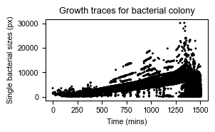
Or, we can plot the growth rate of the total colony over time:
# Get total area of the colony over time
df_sizes_aggregated = df_sizes.groupby(by = ['frame','time'],)['size'].sum().reset_index()

# And plot in log-space
axs = sns.scatterplot(data=df_sizes_aggregated, x="time", y="size",
                      color="black", edgecolor="none", s=5)

axs.set_yscale('log')
# Include doubling rate functions
time_range = np.arange(0,200)
axs.plot(time_range, -1000+5000*2**((time_range)/60), label="Doubling every hour", color='orange')
time_range = np.arange(1400,1600)
axs.plot(time_range, 100*2**((time_range-850)/60), color='orange')
time_range = np.arange(1200,1500)
axs.plot(time_range, 5000*2**((time_range-850)/120), label="Doubling every 2 hours", color='green')
# Legend
axs.legend(loc="lower right")
# Axes limits
axs.set_ylim([np.min(df_sizes_aggregated["size"]), np.max(df_sizes_aggregated["size"])])
# Labels
axs.set_ylabel("Total area (px)")
axs.set_xlabel("Time (min)")
# Title
axs.set_title("Overall colony growth")

# And save
fig = axs.get_figure()
fig.set_size_inches(8.1/2.54, 5/2.54)
plt.tight_layout()
fig.savefig(DATA_FOLDER + "analysis/" + "total_colony_size_over_time.pdf", dpi=300)
plt.show(fig) # for display on workshop website
plt.close(fig)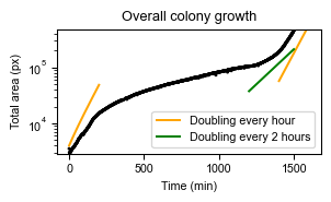
We can now nicely see what happened during the experiment. First, the bacteria were growing relatively fast (doubling ± every hour). Then, antibiotics were added, and growth is substantially slower. Finally, antibiotics are removed, and bacterial growth recovers.
In the previous plot, we can also see the size increase bacteria undergo during antibiotic stress (which was also observed in the original paper).
Note that a more advanced analysis is required to investigate properly what is happening in these experiments. To investigate growth traces of single bacteria, tracking which label corresponds to an individual bacterium over time is required. In addition, the segmentation needs to be of a much higher quality. This could be done by employing manual corrections, or perhaps machine learning techniques could improve segmentation.
KTR data set
As an example, for the KTR dataset, we chose to write scripts in a way such that they can be called directly from the command line.
Script that analyzes the data and creates a csv with data:
""" Analyze KTR data to get C/N ratios

Segments nuclei in KTR data, generates cytoplasmic ROIs,
calculates C/N ratios, and saves the data in a csv file.

Exports a csv file with columns "frame", "KTR_ratio", "int_nucleus", "int_cytoplasm",
where KTR_ratio is the C/N ratio of average cytoplasmic intensity (C) and
average nuclear intensity (N).

Example of how to call script:
python KTR_pipe.py /path/to/Composite_KTR.tif 0 2

With:
- Argument 1: path to the raw KTR data (tif file)
- Argument 2: channel number for nuclear marker (counting starts at 0)
- Argument 3: channel number for KTR sensor (counting starts at 0)

"""

################################################################################
# %% Import libraries

import sys, os
import yaml
import time, datetime
from pathlib import Path

import matplotlib.pyplot as plt
from matplotlib.colors import ListedColormap

import seaborn as sns
import tifffile as tiff
import numpy as np
import pandas as pd

import skimage as sk
from skimage.util import invert

from scipy import stats
from scipy import ndimage

from skimage.measure import label, regionprops
from skimage.feature import peak_local_max

from skimage.morphology import dilation, disk


################################################################################
# %% helper functions for segmentation and analysis

def cmap_random(N):
    """ generate a cmap with random colors (first one black) """
    cmap = np.zeros((N+1, 3))
    for i in range(1, N+1):
        cmap[i] = np.random.rand(3)*0.7 + 0.3
    return ListedColormap(cmap)

def seg_nuclei(input_img):
    """
    Segment nuclei in an image using triangle thresholding.
    """

    # Apply triangle threshold method
    thresh = sk.filters.threshold_triangle(input_img)
    mask = input_img > thresh

    # Remove small objects and label
    mask_filtered = sk.morphology.remove_small_objects(mask, min_size=50)
    result = sk.measure.label(mask_filtered)

    return result


def separate_nuclei(seg_mask, split_distance=5, showplot=False):
    """
    Apply watershed function, based on distance transform.
    See also https://scikit-image.org/docs/0.25.x/auto_examples/segmentation/plot_watershed.html
    """

    # distance transform
    mask_distance = ndimage.distance_transform_edt(seg_mask)

    # blur distance transform to remove noise
    mask_distance_blurred = sk.filters.gaussian(mask_distance, sigma=split_distance/2)

    # find the seeds using local maxima
    local_minima = peak_local_max(mask_distance_blurred,
                                  footprint=disk(split_distance),
                                  exclude_border=False)
    mask_seeds = np.zeros_like(mask_distance, dtype=int)
    mask_seeds[local_minima[:,0], local_minima[:,1]] = 1
    mask_seeds = label(mask_seeds)

    if showplot:
        plt.figure()
        plt.imshow(mask_distance_blurred)
        plt.contour(seg_mask>0, levels=[0.5], colors="r")
        for x,y in local_minima:
            plt.plot(y,x, "ro")
        plt.show()

    # perform watershed
    mask_final = sk.segmentation.watershed(image=-seg_mask,
                                           markers=mask_seeds,
                                           mask=seg_mask>0)

    if showplot:
        plt.figure()
        plt.imshow(mask_final, cmap=cmap_random(200))
        plt.show()

    return mask_final


def get_rings(seg_mask, width=2):
    """ Based on a mask, get areas exactly adjacent to the masks (aka 'rings')

    These areas should correspond to cytoplasm. """

    # dilate to get expanded area
    mask_rings = dilation(seg_mask, disk(width))
    # then remove original to get rings
    mask_rings[seg_mask>0] = 0

    return mask_rings

def get_rings_margin(seg_mask, width=2, margin=1):
    """ Based on mask, get areas directly adjacent to the masks after margin

    These areas should correspond to cytoplasm.
    """

    # dilate to get expanded area (plus margin)
    mask_rings = dilation(seg_mask, disk(width+margin))
    # remove original + margin to get ring around nucleus, with margin
    mask_rings[dilation(seg_mask, disk(margin))>0] = 0

    return mask_rings


# A background correction is requested in a later exercise.
# "correct_bg()" is an example solution.
def correct_bg(img, export_path=None):
    """
    Apply background correction to image.

    Works by determining the mode, and subtracting it.
    Resulting negative values are set to zero.

    If export_path is given, export picture.
    """
    # img = img_KTR; export_path = "/Users/m.wehrens/Desktop/test.png"

    # determine background level and mask
    the_mode = np.bincount(img.ravel()).argmax()
    mask_bg  = img<the_mode

    # subtract it
    img_corr = img - the_mode
    # set would-be negative values to 0
    img_corr[mask_bg] = 0

    if export_path is not None:

        fig, axs = plt.subplots(1,3, figsize=(15/2.54,5/2.54))
        plt.rcParams.update({"font.family": "Arial", "font.size": 7})

        # Show image, and image with identified background pixels
        axs[0].imshow(img)
        axs[1].imshow(img)
        axs[1].imshow(mask_bg, alpha=mask_bg*1.0)

        # show it in the histogram
        axs[2].hist(img.ravel(), bins=32, color='grey')
        axs[2].axvline(the_mode, color='red')
        axs[2].set_xlabel("Intensity")
        axs[2].set_ylabel("Counts")

        plt.tight_layout()
        fig.savefig(export_path, dpi=600)
        plt.close()

    return img_corr


def get_mean_intensity(img, mask):
    """Calculate means in areas corresponding to labeled mask in image img."""

    # Calculate totals per index
    sums   = np.bincount(mask.ravel(), weights=img.ravel())
    # Calculate pixel coverage per index
    counts = np.bincount(mask.ravel())

    # Calculate the means
    return (sums/counts)[1:]

################################################################################
# %% Code executed when script is called

if __name__ == "__main__":

    # Input arguments
    img_path_KTR = sys.argv[1]
    channel_nuc = int(sys.argv[2])
    channel_ktr = int(sys.argv[3])

    # Set up an output directory named "analysis" in the parent directory
    # (This assumes the raw data is stored in its own subdirectory in sample folder)
    # e.g.
    # ../../projectX/data/sampleXYZ_202606/raw/
    # ../../projectX/data/sampleXYZ_202606/analysis/
    output_dir = Path(os.path.dirname(img_path_KTR)).parent / "analysis"
    os.makedirs(output_dir, exist_ok=True)
    path_bg_fig = os.path.join(output_dir, f"background_correction_{channel_ktr}.png")

    # Load data
    # img_path_KTR = '/Users/m.wehrens/Data_notbacked/2025_Py-Image-workshop_KTR-example-data/raw/Composite_KTR.tif'
    # channel_nuc = 0; channel_ktr = 2
    KTR_data = tiff.imread(img_path_KTR)

    # Initialize empty list to store dataframes
    df_KTR_list = [None]*KTR_data.shape[0]
    # Loop over the frames
    for fr_idx in range(0, KTR_data.shape[0]):
        # fr_idx=0

        print(f"Working on frame {fr_idx} / {KTR_data.shape[0]}")

        # get nuclei and KTR intensity images
        img_nuc = KTR_data[fr_idx, channel_nuc, :, :]
        img_KTR = KTR_data[fr_idx, channel_ktr, :, :]
            # plt.imshow(img_nuc)
            # plt.imshow(img_KTR)

        # correct the background (requested in later exercise)
        if fr_idx == 0:
            # if first frame, also export image to check whether
            # background correction was appropriate
            img_KTR = correct_bg(img_KTR, export_path=path_bg_fig)
        else:
            img_KTR = correct_bg(img_KTR)

        # Calculate the mask
        mask_nuclei       = seg_nuclei(img_nuc)
        mask_nuclei_split = separate_nuclei(mask_nuclei, split_distance=5)

        # Calculate averages
        KTR_means_nucl = get_mean_intensity(img_KTR, mask_nuclei_split)
        KTR_means_cyto = get_mean_intensity(img_KTR, get_rings_margin(mask_nuclei_split))
            # plt.imshow(get_rings(mask_nuclei_split), cmap=cmap_random(200))
            # CM = cmap_random(200); plt.imshow(mask_nuclei_split, cmap=CM); plt.imshow(get_rings_margin(mask_nuclei_split), cmap=CM, alpha=(get_rings_margin(mask_nuclei_split)>1)*1.0)

        # Get ratio
        KTR_ratios = KTR_means_cyto/KTR_means_nucl

        # Store the data
        df_KTR_list[fr_idx] = pd.DataFrame({
            "frame": fr_idx,
            "KTR_ratio": KTR_ratios,
            "int_nucleus": KTR_means_nucl,
            "int_cytoplasm": KTR_means_cyto
        })

    # Now merge the dataframes
    df_KTR = pd.concat(df_KTR_list, ignore_index=True)

    # Save data to csv
    output_path = os.path.join(output_dir, f"KTR_ratios_ch{channel_ktr}.csv")
    df_KTR.to_csv(output_path, index=False)
    print(f"Data saved to {output_path}")


# %%

if __name__ == "main":

    """
    python KTR_pipe.py /Users/m.wehrens/Data_notbacked/2025_Py-Image-workshop_KTR-example-data/raw/Composite_KTR.tif 0 2
    """
Creating a plot based on the csv:
"""Creates plot of ratios from csv file

Example usage:
python KTR_plot.py /path/to/KTR_ratios_ch1.csv 25

With:
- First argument: path to the csv file created by KTR_pipe.py
- Optional second argument: time of stimulation in minutes (plotted as vertical line)
"""

################################################################################
# %% Import libraries

import sys, os
from pathlib import Path
import pandas as pd
import seaborn as sns

import matplotlib.pyplot as plt

################################################################################
# %% plotting function

def plot_data(DATA_PATH, stim_time = None):

    # Get relevant path information
    OUTPUT_DIR = Path(DATA_PATH).parent
    FILENAME   = Path(DATA_PATH).stem

    # Read the data
    df_KTR = pd.read_csv(DATA_PATH)

    # add time field
    # From the image metadata: Frame interval: 270.01617 sec
    df_KTR['time_s'] = 270.01617 * df_KTR['frame'] / 60

    # Now plot the data
    plt.rcParams["font.family"] = "Arial"
    plt.rcParams["font.size"] = 8
    fig, axs = plt.subplots(1,1, figsize=(5/2.54,5/2.54))
    sns.scatterplot(df_KTR, x="time_s", y="KTR_ratio", ax=axs,
                    color="k", alpha=0.05, s=5, edgecolor=None)
    sns.lineplot(df_KTR, x="time_s", y="KTR_ratio", estimator="mean", color="r", ax=axs)
    if stim_time is not None:
        axs.axvline(stim_time, color="b", ls="--")
    axs.set_xlabel("Time (min)")
    axs.set_ylabel("Sensor C/N ratio")
    axs.set_ylim(0, 1.5)
    plt.tight_layout()

    # save to same directory
    output_path_fig = os.path.join(OUTPUT_DIR, f"{FILENAME}_overtime.png")
    fig.savefig(output_path_fig, dpi=600)

    plt.close(fig)


################################################################################
# %% Code that gets executed when script is called

if __name__ == "__main__":

    # DATA_PATH = "/Users/m.wehrens/Data_notbacked/2025_Py-Image-workshop_KTR-example-data/analysis/KTR_ratios_ch1.csv"
    # STIM_TIME = 25

    # Read input arguments
    DATA_PATH = sys.argv[1]
    if len(sys.argv) > 2:
        STIM_TIME = int(sys.argv[2])

    # Make plot
    plot_data(DATA_PATH, stim_time=STIM_TIME)

    # python KTR_plot.py /Users/m.wehrens/Data_notbacked/2025_Py-Image-workshop_KTR-example-data/analysis/KTR_ratios_ch2.csv 25
These scripts can be called from the command line. Navigate to the directory with the scripts and call:
# To perform the analysis:
python KTR_pipe.py /path/to/Composite_KTR.tif 0 2

# To create the plot:
python KTR_plot.py /path/to/KTR_ratios_ch1.csv 25