import matplotlib.pyplot as plt
import seaborn as sns
import tifffile as tiff
import numpy as np

import skimage as sk
from scipy import stats
from scipy import ndimage

from skimage.measure import label, regionprops

def my_plot_1(img1, mycmap='gray', myfigsize=(5/2.54,5/2.54)):
    fig, ax = plt.subplots(1,1, figsize=myfigsize)
    _=plt.imshow(img1, cmap=mycmap)

def my_plot_12(img1, img2, mycmap='viridis', myfigsize=(10/2.54,5/2.54)):
    # plot two images side by side
    fig, axs = plt.subplots(1,2, figsize=myfigsize)
    _ = axs[0].imshow(img1, cmap=mycmap)
    _ = axs[1].imshow(img2, cmap=mycmap)
plt.tight_layout() Workshop Python Image Analysis
Martijn Wehrens, May 2026
Answers to exercises 03
Creating segmentation functions
def seg_bacterium(input_img):
"""
Segment bacteria in an image using LoG zero crossings and watershed.
"""
# input_img = np.max(img_ecoli)-img_ecoli
# Smooth image before Laplacian filtering
img_gauss = sk.filters.gaussian(input_img, sigma=3)
edges_log = sk.filters.laplace(img_gauss)
# minmaxval = np.max(np.abs(edges_log)); plt.imshow(edges_log, cmap='bwr', vmin=-minmaxval, vmax=minmaxval)
# Identify LoG zero crossings as bacterial outlines
edges_min = ndimage.minimum_filter(edges_log, footprint=sk.morphology.disk(1))
edges_max = ndimage.maximum_filter(edges_log, footprint=sk.morphology.disk(1))
mask_edges = np.logical_and(edges_min < 0, edges_max > 0)
# plt.imshow(mask_edges)
# Build a whole-colony mask from triangle thresholding
mask_triangle = input_img > sk.filters.threshold_triangle(input_img)
mask_triangle = sk.morphology.remove_small_objects(mask_triangle, min_size=50)
mask_triangle = sk.morphology.dilation(mask_triangle, footprint=sk.morphology.disk(8))
# plt.imshow(mask_triangle)
# Restrict edges to the colony and fill enclosed bacteria
mask_edges = np.logical_and(mask_edges, mask_triangle)
mask_filled = ndimage.binary_fill_holes(mask_edges)
# plt.imshow(mask_filled)
# Erode to create separated seed regions for watershed
mask_seeds = sk.morphology.erosion(mask_filled, footprint=sk.morphology.disk(4))
mask_seeds = sk.measure.label(mask_seeds)
# plt.imshow(mask_seeds)
# Expand seeds back into the filled bacterial mask
result = sk.segmentation.watershed(-1 * mask_filled, markers=mask_seeds, mask=mask_filled)
# plt.imshow(result)
return result
def seg_nuclei(input_img):
"""
Segment nuclei in an image using triangle thresholding.
"""
# Apply triangle threshold method
thresh = sk.filters.threshold_triangle(input_img)
mask = input_img > thresh
# Remove small objects and label
mask_filtered = sk.morphology.remove_small_objects(mask, min_size=50)
result = sk.measure.label(mask_filtered)
return result
# Now let's test the above functions
# Bacteria
img_ecoli = tiff.imread('../images/biological/microcolony_ecoli.tif')
mask_bacteria = seg_bacterium(np.max(img_ecoli)-img_ecoli)
_ = plt.imshow(mask_bacteria)
plt.show()
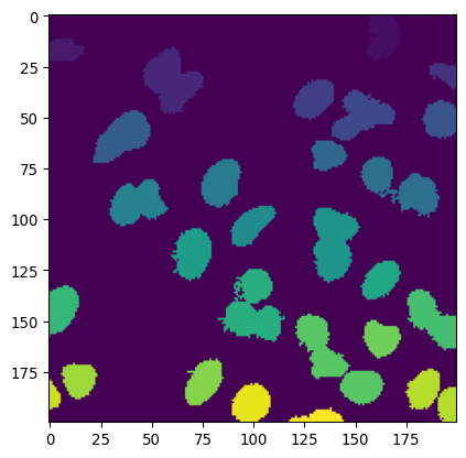
# Nuclei
img_path_KTR = '/Users/m.wehrens/Data_notbacked/2025_Py-Image-workshop_KTR-example-data/raw/Composite_KTR.tif'
img_nuclei = tiff.imread(img_path_KTR)[0, 0, 0:200, 0:200]
mask_nuclei = seg_nuclei(img_nuclei)
_ = plt.imshow(mask_nuclei)
plt.show()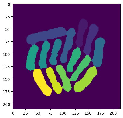
Counting spots
# Read the image
img_spots = tiff.imread("../images/bioimagebook/spots.tif")
_ = plt.title("Original spots image")
_ = plt.imshow(img_spots)
plt.show()
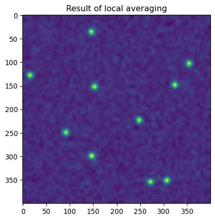
# Create a local mean convolution kernel
a_disk = sk.morphology.disk(5)
the_kernel = a_disk/np.sum(a_disk)
# Apply it to the image `images/bioimagebook/spots.tif`.
img_spots_convolved = ndimage.convolve(img_spots, the_kernel)
# Show the result
_ = plt.title("Result of local averaging")
_ = plt.imshow(img_spots_convolved)
plt.show()
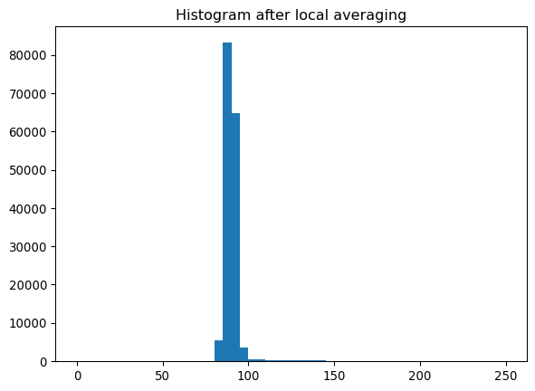
_ = plt.title("Histogram after local averaging")
_ = plt.hist(img_spots_convolved.ravel(), bins = np.arange(0, 255, 5))
plt.show()
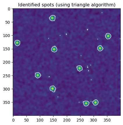
# Segment based on new image
threshold_triangle = sk.filters.threshold_triangle(img_spots_convolved)
mask_spots = img_spots_convolved > threshold_triangle
# Make a plot with contours
_ = plt.title("Identified spots (using triangle algorithm)")
_ = plt.imshow(img_spots_convolved)
_ = plt.contour(mask_spots, colors='w', linewidths=1, levels=[0.5])
plt.show()
# Count the spots
regionprops_spots = regionprops(label(mask_spots))
areas_spots = np.array([r.area for r in regionprops_spots])
# Let's count a spot if area>3
print("Total nr of spots:", np.sum(areas_spots>3))
# In case we're perfectionists
# Using a relative margin of 0.2
# Similar as to what is done in Zack et al. in 1977. (https://doi.org/10.1177/25.7.7045)
img_mode = np.bincount(img_spots_convolved.ravel()).argmax()
img_max = np.max(img_spots_convolved)
threshold_margin = (img_max-img_mode)/5
mask_spots2 = img_spots_convolved > (threshold_triangle+threshold_margin)
rprops_spots2 = regionprops(label(mask_spots2))
# And plot
_ = plt.title('Identified spots (triangle, using "Zack" margin)')
_ = plt.imshow(img_spots_convolved)
_ = plt.contour(mask_spots2, colors='w', linewidths=1, levels=[0.5])
# add labels
for i, r in enumerate(rprops_spots2):
minr, minc, maxr, maxc = r.bbox
_ = plt.text(maxc+5, maxr, str(i+1), color='w')
plt.show()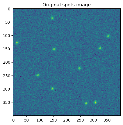
Total nr of spots: 10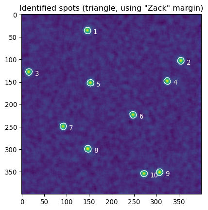
License plate
img_shady = tiff.imread('../images/car/chatGPT_shadybusiness_licensehigh-8bit.tif')
img_shady_inv = np.max(img_shady)-img_shady
my_plot_1(img_shady_inv, mycmap='viridis')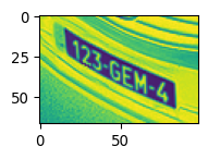
# Segment the symbols on the license plate

# apply triangle thresholding
thresh = sk.filters.threshold_otsu(img_shady_inv)
# get the mask
mask_shady = img_shady_inv>thresh
mask_shady_labeled = sk.measure.label(mask_shady)
props_shady = sk.measure.regionprops(mask_shady_labeled)
# retain labels that are >10, <100 in area
mask_shady_filt = np.isin(mask_shady_labeled,
                          [p.label for p in props_shady if p.area>5 and p.area<200])

# show result
my_plot_12(mask_shady, mask_shady_filt, mycmap='gray')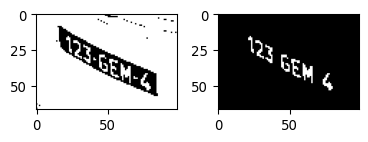
# acquire labels and regionprops
mask_shady_filt_label = sk.measure.label(mask_shady_filt)
props_shady = sk.measure.regionprops(mask_shady_filt_label)

# plot every bbox separately
fig, axs = plt.subplots(1,len(props_shady), figsize=(len(props_shady)*5/2.54,5/2.54))
for i, p in enumerate(props_shady):
    minr, minc, maxr, maxc = p.bbox
    # Plot (and remove axes)
    _ = axs[i].imshow(img_shady_inv[minr:maxr, minc:maxc], cmap='magma')
    axs[i].axis('off')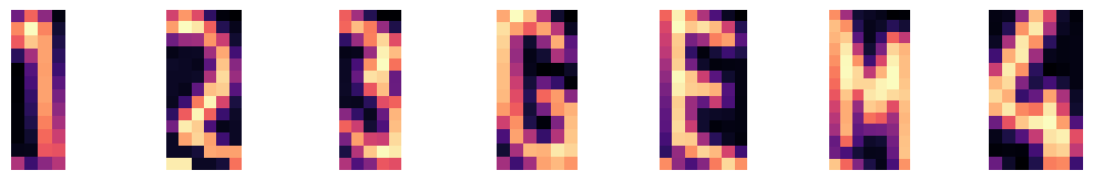
Distance transform
# load images
img_path_KTR = '/Users/m.wehrens/Data_notbacked/2025_Py-Image-workshop_KTR-example-data/raw/Composite_KTR.tif'
img_nuclei = tiff.imread(img_path_KTR)[0, 0, 0:200, 0:200]

# Let's also load an image of some bacteria (Wehrens et al.)
path_img_ecoli = '../images/biological/microcolony_ecoli.tif'
img_ecoli = tiff.imread(path_img_ecoli)
img_ecoli_inv = np.max(img_ecoli)-img_ecoli # invert image

# create mask
mask_nuclei_triangle = img_nuclei > sk.filters.threshold_triangle(img_nuclei)
mask_ecoli_triangle = img_ecoli_inv > sk.filters.threshold_triangle(img_ecoli_inv)
# Perform a distance perform on the bacterial image
distance_nuclei = ndimage.distance_transform_edt(mask_nuclei_triangle)
distance_ecoli = ndimage.distance_transform_edt(mask_ecoli_triangle)
# Show it
fig, axs = plt.subplots(1,2)
_=axs[0].imshow(distance_nuclei, cmap='magma')
_=axs[1].imshow(distance_ecoli, cmap='magma')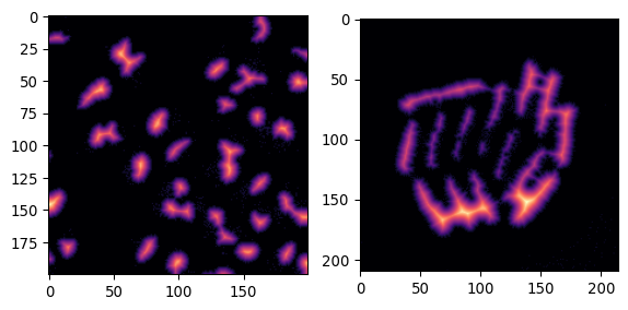
# Get local maxima for the nuclei
local_max_nuclei = sk.feature.peak_local_max(distance_nuclei,
                                             min_distance = 10,
                                             threshold_abs = 3,
                                             footprint=sk.morphology.disk(10),
                                             exclude_border=False)

# Plot the nuclei picture, and plot the local maxima on top as crosses
fig, ax = plt.subplots()
_ = ax.imshow(img_nuclei, cmap='viridis')
x = local_max_nuclei[:, 1]
y = local_max_nuclei[:, 0]
_ = ax.plot(x, y, 'r+')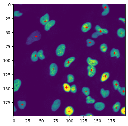
Thus, the local maxima correspond relatively well to individual nuclei. This could be used in further processing (watershedding) to separate them.
Another approach to identify individual nuclei is to erode the mask that was found, in the hope that for nuclei that are connected only a little, the connection gets eroded away.