Workshop Python Image Analysis

Martijn Wehrens, September 2025

Answers to exercises 03

# libraries
import numpy as np
import tifffile as tiff
import matplotlib.pyplot as plt
import skimage as sk
import scipy

Exercise answers

E. moji

image_path = '../images/emoji/emojis-swimming.tif'
img_emoji = tiff.imread(image_path)

_ = plt.imshow(img_emoji)
plt.show()

# Try to segment the "E. moji" image, both the *E. mojis* and the other organism (*S. hark*?) that are present.

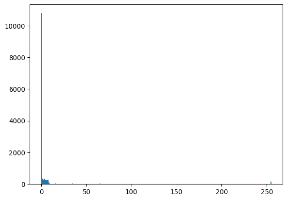
# Let's inspect a histogram first
_ = plt.hist(img_emoji.ravel(), bins=256)
plt.show()

# The peak at 0 is probably background, so simply create mask >0
mask_emoji = img_emoji>0
_ = plt.title("Rudimentary.")
_ = plt.imshow(mask_emoji)
plt.show()

# Optionally, we can remove holes
_ = plt.title("Masks covering the complete objects.")
mask_emoji_noholes = scipy.ndimage.binary_fill_holes(mask_emoji)
_ = plt.imshow(mask_emoji_noholes)
plt.show()

# Make a histogram of the object sizes.
labelmask_emoji = sk.measure.label(mask_emoji)
rprops_emoji    = sk.measure.regionprops(labelmask_emoji)
_ = plt.title("Size histogram (red = uncorrected, blue = corrected).")
_ = plt.hist([r.area for r in rprops_emoji], bins=100, color='red')
_ = plt.xlim([0,1000])
# (optionally) add another histogram for the no-holes version
labelmask_emoji_noholes = sk.measure.label(mask_emoji_noholes)
rprops_emoji_noholes    = sk.measure.regionprops(labelmask_emoji_noholes)
_ = plt.hist([r.area for r in rprops_emoji_noholes], bins=100, color='blue')
# show
plt.show()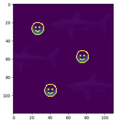

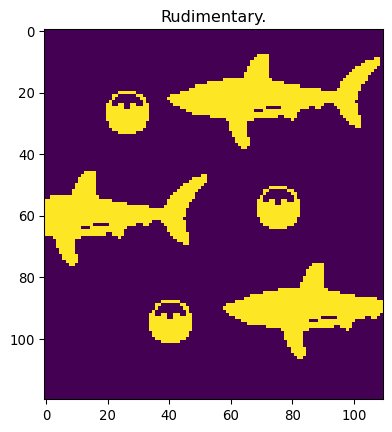
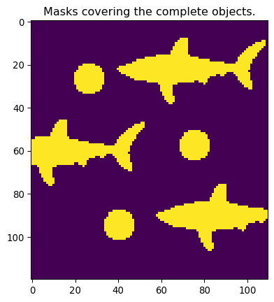
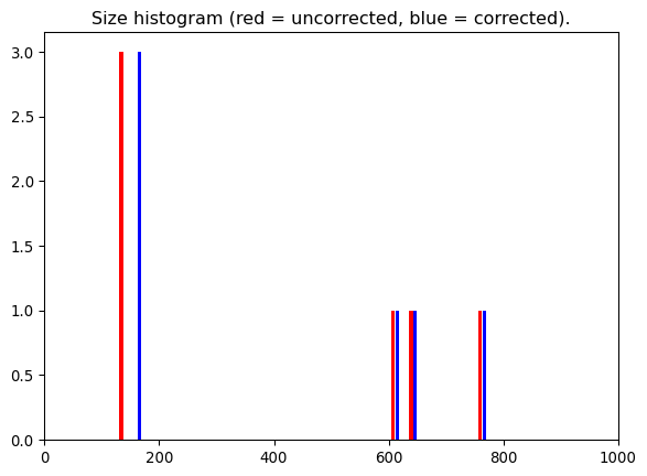
Why does the histogram look the way it does? Let’s first recognize that without the hole-filling, we cannot create a really truthfull mask based on the thresholding alone.

The values in the histogram reflect the size of the different objects. The smiley-faces all have the same object size, hence the big peak. But all the sharks will show a different size, hence the three smaller peaks.

Nuclei

# We made a histogram of nuclear sizes, but the sizes were in pixels. Produce a histogram with the sizes in microns. (You might need a tool like FIJI.)

# Let's reiterate creating the mask and collecting the sizes
img_path_KTR = '/Users/m.wehrens/Data_notbacked/2025_Py-Image-workshop_KTR-example-data/raw/Composite_KTR.tif'
img_nuclei = tiff.imread(img_path_KTR)[0, 0, 0:200, 0:200]
_ = plt.imshow(img_nuclei, cmap='magma')
plt.show()

# Get mask and region properties
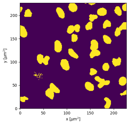
mask_nuclei = img_nuclei>700
labeled_nuclei = sk.measure.label(mask_nuclei)
regions = sk.measure.regionprops(labeled_nuclei, intensity_image=img_nuclei)

# From the metadata, we learn the following
pixel_length = 1.1364
pixel_area   = pixel_length**2

# Show the mask for reference
_ = plt.imshow(
        mask_nuclei, 
        extent = [0, mask_nuclei.shape[1]*pixel_length, 
                  0, mask_nuclei.shape[0]*pixel_length], 
        origin='lower'
    )
_ = plt.xlabel(f"x [$\\mu m^2$]")
_ = plt.ylabel(f"y [$\\mu m^2$]")
plt.show()

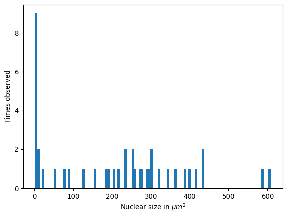
# Now produce a histogram with the real sizes
_ = plt.hist([r.area*pixel_area for r in regions], bins=100)
_ = plt.xlabel(f"Nuclear size in $\\mu m^2$")
_ = plt.ylabel("Times observed")
plt.show()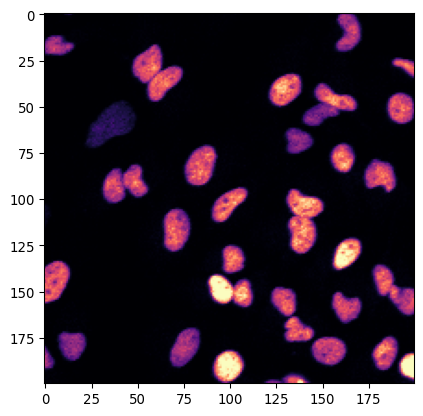

# Can you also add their contours?

# Let's add contours to the original image
_ = plt.imshow(img_nuclei, cmap='magma')
_ = plt.contour(
        mask_nuclei, 
        levels = [0.5],
        colors='lightblue',
    )
# And put a cross in their centers
centroids = np.array([r.centroid for r in regions])
_ = plt.plot(centroids[:,1], centroids[:,0], 'xw')
    
plt.show()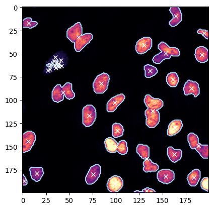

# And now for the color map that clearly shows the mask

# Use the functions `np.random.rand()` and `ListedColormap()` to create a colormap that's a bit more useful to display the labeled nuclei.

from matplotlib.colors import ListedColormap

# Create a random colormap for labeled nuclei
colors = (np.random.rand(len(regions) + 1, 3)+.2)/1.2
colors[0] = [0, 0, 0]  # Background is black
cmap = ListedColormap(colors)

# Display labeled nuclei with the random colormap
_ = plt.imshow(labeled_nuclei, cmap=cmap)
plt.show()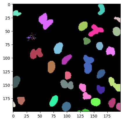

Optional exercises answers

import matplotlib.pyplot as plt
import seaborn as sns
import tifffile as tiff
import numpy as np

import skimage as sk
from scipy import stats
from scipy import ndimage

# Dodgy guys

# Load the picture `images/car/dodgy-guys.tif`
img_dodgy = tiff.imread('../images/car/dodgy-guys.tif')
_=plt.imshow(img_dodgy)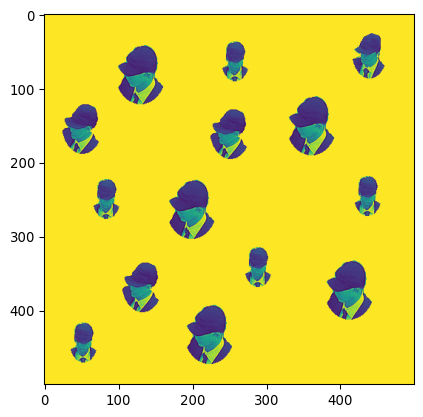

# Can you count the amount of dodgy guys with python?
mask_dodgy_inv = np.max(img_dodgy)-img_dodgy
mask_dodgy = mask_dodgy_inv>2
labeledmask_dodgy = sk.measure.label(mask_dodgy)
np.max(labeledmask_dodgy)

np.int32(14)

# Can you identify where they are in the image (put a cross in a plot)?
regions_dodgy = sk.measure.regionprops(labeledmask_dodgy)
centroids_dodgy = np.array([r.centroid for r in regions_dodgy])
_=plt.imshow(img_dodgy)
_=plt.plot(centroids_dodgy[:,1], centroids_dodgy[:,0], 'xr')
# Can you put the sizes of each of the heads on top of their heads in a plot?
sizes_dodgy = np.array([r.area for r in regions_dodgy])
for i, size in enumerate(sizes_dodgy):
    plt.text(centroids_dodgy[i,1]+10, centroids_dodgy[i,0], str(round(size)), color='red')

# Can you now easily spot which of the faces only occurs once in this image?
np.unique(sizes_dodgy, return_counts=True)

(array([1261., 1743., 2324., 3381.]), array([5, 1, 3, 5]))

So the face corresponding to size 1743 occurs only once.