Workshop Python Image Analysis

Martijn Wehrens, September 2025

Answers to exercises 02

import matplotlib.pyplot as plt
import seaborn as sns
import tifffile as tiff
import numpy as np

img_path = '../images/car/chatGPT_shadybusiness_zoomhigh-custom.tif'
img = tiff.imread(img_path)

_ = plt.imshow(img)

# From the image below, you can estimate the 
# coordinates of the license plate.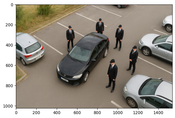

_ = plt.imshow(img[710:770, 430:520])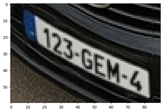

image_path2 = '../images/car/chatGPT_shadybusiness_zoomlow-8bit.tif'

img_small = tiff.imread(image_path2)
fig, ax = plt.subplots()
_= ax.imshow(img_small, cmap='grey')
rect = plt.Rectangle((107,177), 23, 15,
                     # (x, y), width, height
                  linewidth=3, edgecolor='r', 
                  facecolor='none')
_ = ax.add_patch(rect)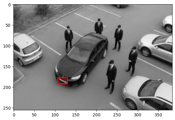

_ = plt.imshow(img_small[710//4:770//4, 430//4:520//4], cmap='grey')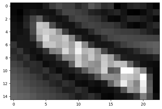

Clearly, there is not enough information in this image to read the license plate.

# Different cmaps
# Google for "python cmap"
# Find: https://matplotlib.org/stable/users/explain/colors/colormaps.html

fig, ax = plt.subplots(3,2)
_= ax[0,0].imshow(img_small, cmap='grey')
_= ax[0,0].set_title('cmap=grey')
_= ax[1,0].imshow(img_small, cmap='viridis')
_= ax[1,0].set_title('cmap=viridis')
_= ax[2,0].imshow(img_small, cmap='plasma')
_= ax[2,0].set_title('cmap=plasma')
_= ax[0,1].imshow(img_small, cmap='jet')
_= ax[0,1].set_title('cmap=jet')
_= ax[1,1].imshow(img_small, cmap='hsv')
_= ax[1,1].set_title('cmap=hsv')
_= ax[2,1].imshow(img_small, cmap='Dark2')
_= ax[2,1].set_title('cmap=Dark2')
plt.tight_layout()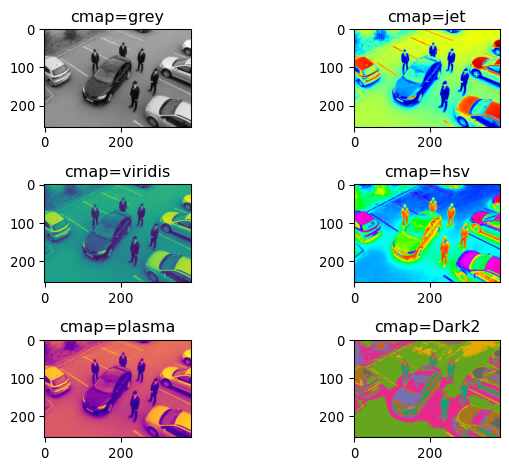

Perceptually uniform

Note that viridis and plasma are perceptually uniform color maps, meaning that a specific value difference will look the same indepedent of the location on the scale.

This is an important feature, as otherwise you might see contrasts that are not really there.

Adding 100

img_small_plus100 = img_small+100
_=plt.imshow(img_small_plus100, cmap='grey')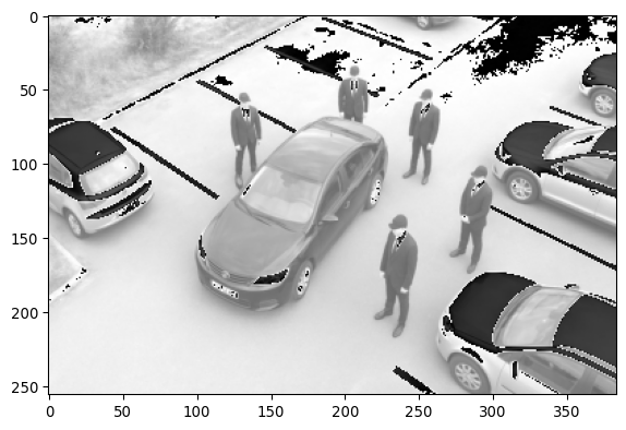

fig, ax = plt.subplots(2,1)
_=ax[0].hist(img_small.ravel(), bins=255)
_=ax[0].axvline(x=255-100, color='r', linestyle='-')
_=ax[1].hist(img_small_plus100.ravel(), bins=255)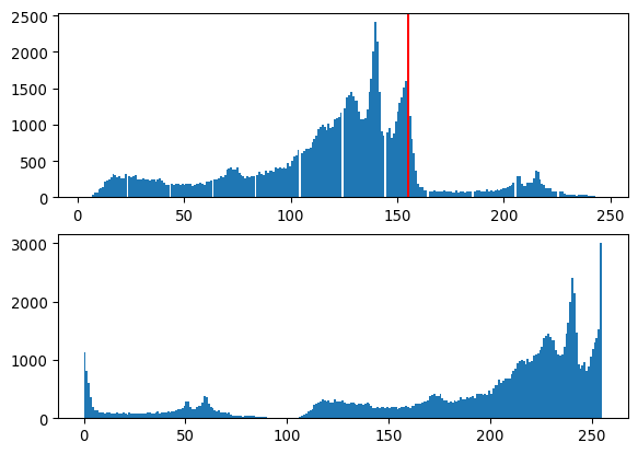

The values can only take values between 0-255, so if we add 100, values >255 are put back in that scale in a periodic fashion. (E.g. 160+100 = 4, or 260-256, consistent with there only being 256 values available.)

Additional exercises

# Read the KTR image
img_path_KTR = '/Users/m.wehrens/Data_notbacked/2025_Py-Image-workshop_KTR-example-data/raw/Composite_KTR.tif'
img_KTR = tiff.imread(img_path_KTR)

# Display a histrogram of the first channel (t=0)
_ = plt.hist(img_KTR[0,0,:,:].ravel())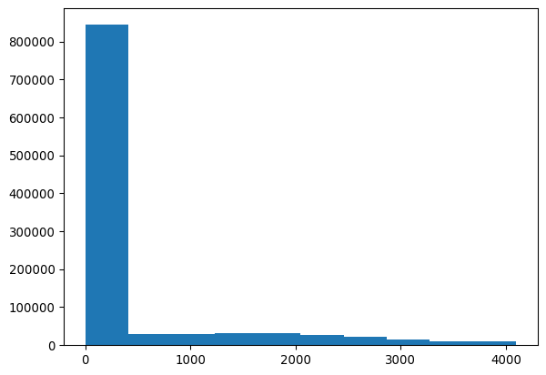

# Determine a threshold, based on the histogram
MY_THRESHOLD = 2000

# Display the binary thresholed image
img_nuclei = img_KTR[0,0,0:200,0:200]
_ = plt.imshow(img_nuclei>MY_THRESHOLD)

# Save the mask
img_nuclei_thresholded = \
    img_nuclei>MY_THRESHOLD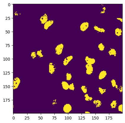

# Display both the original nuclei and the mask
_ = plt.imshow(img_nuclei)
_ = plt.contour(img_nuclei_thresholded, 
                levels=[0.5], colors='red')
                # levels determines at which level to draw isolines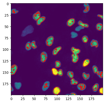

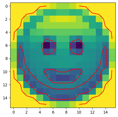
# Additional contour example

# Load the :-) image
image_path_smile = '../images/emoji/emoji-8bit-gray.tif'
img_smile = tiff.imread(image_path_smile)

# Show the image and contours
_ = plt.imshow(img_smile)
_ = plt.contour(img_smile, levels=[150,250], colors='red')