import torch
from torch import nn

from torch.utils.data import Dataset

import numpy as np

import tifffile as tiff
import matplotlib.pyplot as pltWorkshop Python Image Analysis
Martijn Wehrens, September 2025
Estimated time: 20 mins presenting + 60 mins exercises + 20 mins discussion
Chapter 6: A very basic introduction into machine learning
Pytorch required
Code in this notebook might need to be run on Google colab or the like, as laptops might not have the right architecture to run the required pytorch library.
Outline of this mini-workshop
This chapter introduces quite some concepts, and is sometimes a bit concise. It is intended to be combined with questions or discussions with an instructor that is present.
- Mini lecture about Machine Learning
- /Users/m.wehrens/Documents/PRESENTATIONS/TEACHING/ML_verybasic.pptx
- Go over the questions in this notebook
- Don’t try to understand all code!
Exercise: draw 4 images
Open FIJI and create a new 12x12 8bit image. Use the paintbrush tool and color picker to draw four images. Draw 2 images depicting one thing, and two images depicting another thing. E.g. draw 2 images of an apple and two images of a pear. Only spend a few minutes on this. (You can also draw something easier, like numbers, symbols, letters, etc.)
Run some code
The code below uses pytorch to set up a very simple neural network. “Real” neural networks have a much more complicated architecture. The purpose here is to be able to follow along what’s happening in a neural network.
Understanding, but not the technical details
The code has some explanatory comments, but it takes too much time to explain fully how pytorch or similar neural network libraries (like tensorflow or keras) work. You’re welcome to try and understand the code, but don’t get lost in it, the main goal is to understand the concepts of machine learning.
# Technical note: ".to(DEVICE)" tells the computer to run this
# neural network on a specific architecture, which enables
# faster calculations.
#
# Common options:
    # CPU: .to("cpu")
    # NVIDIA GPU: .to("cuda") or .to("cuda:0")
    # Apple GPU via Metal: .to("mps")
    # Intel GPU with supported PyTorch build: .to("xpu")

DEVICE = 'mps'
# This code defines a VERY simple model for 12x12 pixels,
# meant for illustratory purposes.
class VerySimpleNN(nn.Module):
# Pytorch makes use of classes, which are a way to group
# data and functions together. A class specifies what functions
# the class provides, and what data (like parameters) it stores.
# An object can then be created to actually load data and
# call those functions.
# As an analogy, class definitions are the "blueprint",
# objects instantiated from the class are the "houses".
#
# Here, we define a class (blueprint) for our simple
# neural network.
#
# To learn more about classes, e.g. google for a tutorial on
# Python classes.
def __init__(self):
# __init__ is a standard class method, which is
# automatically called when an object is created.
#
# In this case, it defines how (the layers
# of) the network should look.
# technical; calls init of parent class
super().__init__()
# Define a flatten function, which in this case
# can flatten the input (the image) to a 144 element vector
self.flatten = nn.Flatten()
# Define a linear layer, which will
# calculate weights*pixels for 144 element input and 2 output elements
self.linear = nn.Linear(12*12, 2)
def forward(self, x):
# The forward function can be called later to actually
# generate a prediction.
# It will use the "components" we defined in __init__.
# (This is useful when the network is more complicated,
# and more complex structures or components are defined in __init__, and
# the forward function will be less complex.)
# Now actually use the flatten function to convert
# the 12x12 input to a 1d 144 long vector.
x = self.flatten(x)
# technical note:
# typically, input will be supplied in batches,
# so the input shape will be (batchsize, 12, 12)
# and the output shape will be (batchsize, 144)
# Now use the linear layer to calculate the 2 element output
logits = self.linear(x)
return logits
###
# Now test the neural network
# Instantiate the neural network (create an object from the class)
simpleNN = VerySimpleNN().to(DEVICE)
# Generate a random 12x12 image
test_data = torch.rand(1, 12, 12, device=DEVICE)
print('test_data=',test_data)
# Generate a prediction; calling the object will automatically
# call the forward function (since this is a pytorch class)
# Alternatively, you could also call simpleNN.forward(test_data)
pred = simpleNN(test_data)
pred_numpy = pred.cpu().detach().numpy()
# Print the prediction
print('pred = \"',pred, '\" (pytorch tensor format)')
print('pred_numpy = \"',pred_numpy,'\" (numpy format)')test_data= tensor([[[0.9009, 0.8022, 0.0475, 0.2212, 0.2600, 0.2308, 0.0562, 0.6480,
0.1600, 0.2574, 0.2358, 0.1446],
[0.6342, 0.3485, 0.8966, 0.7321, 0.8023, 0.3730, 0.8979, 0.4785,
0.1898, 0.5224, 0.9702, 0.4104],
[0.6250, 0.3639, 0.9362, 0.6310, 0.1274, 0.3194, 0.9687, 0.8369,
0.6619, 0.8533, 0.9156, 0.0776],
[0.0375, 0.5412, 0.1547, 0.5569, 0.9840, 0.2482, 0.4367, 0.2520,
0.8260, 0.0903, 0.7654, 0.8998],
[0.0614, 0.6663, 0.2172, 0.5770, 0.9063, 0.2243, 0.0469, 0.7821,
0.1072, 0.9495, 0.4456, 0.0303],
[0.5431, 0.9573, 0.8628, 0.7446, 0.1259, 0.1274, 0.8468, 0.3019,
0.5827, 0.7253, 0.3702, 0.7132],
[0.4580, 0.4030, 0.0668, 0.0687, 0.3347, 0.6244, 0.1637, 0.3826,
0.4348, 0.7631, 0.0950, 0.8594],
[0.4877, 0.1121, 0.4675, 0.8743, 0.8862, 0.7936, 0.5068, 0.6614,
0.7893, 0.1848, 0.6366, 0.5639],
[0.7879, 0.5979, 0.6778, 0.0065, 0.6370, 0.9467, 0.5627, 0.5850,
0.7445, 0.4278, 0.1157, 0.3201],
[0.4365, 0.8525, 0.3081, 0.2557, 0.2749, 0.2713, 0.2122, 0.1717,
0.3923, 0.8705, 0.8611, 0.9386],
[0.5581, 0.5787, 0.7713, 0.8367, 0.0725, 0.6568, 0.0481, 0.8928,
0.4136, 0.1494, 0.5207, 0.1778],
[0.9819, 0.3049, 0.4852, 0.9620, 0.0038, 0.7785, 0.6383, 0.9068,
0.9004, 0.5349, 0.6441, 0.1906]]], device='mps:0')
pred = " tensor([[0.3417, 0.2558]], device='mps:0', grad_fn=<LinearBackward0>) " (pytorch tensor format)
pred_numpy = " [[0.34165448 0.25576425]] " (numpy format)Remarks: Tensors
As you can see the output has the type tensor. This is an internal data structure of pytorch, which is similar to a numpy array. The reason we’re using these ‘special’ arrays is (1) that their technical setup allows for calculating the “gradient” (\(\delta\text{loss}/\delta w\)) used to update the weights \(w\) and (2) they can be put on GPUs, which can speed up calculations a lot.
Questions
- What role does \(\delta\text{loss}/\delta w\) play in neural networks?
- This questions regards the code under the heading “# Now test the neural network” above. Can you describe in your own terms what
- The input we give to the network looks like here?
- What the output of the neural network looks like?
- If we were to provide actual images to this network, do you think it would be able to generate meaningful predictions? Why would it (not)?
Concise answers
- \(\delta\text{loss}/\delta w\) is the gradient, which indicates in which direction the weights should be adjusted to reduce the loss.
- This network expects 12x12 images, the input we give here is just random values in the correct shape. The output is an array corresponding to each of the classes, with a respective score that reflects to what extend the input matched that class. In our example [score_happy, score_sad]. Whichever value is the highest, is the predicted class. The output now shows random numbers since the input as well as the weights had random values.
- No, since the weights are not set during a training setting yet.
# Since this network is so simple, we can manually calculate it's outcome

# Now acquire the weights stored in the neural network
# And convert them from tensors to numpy
weights = simpleNN.linear.weight.detach().cpu().numpy()
bias    = simpleNN.linear.bias.detach().cpu().numpy()
    # bias is a constant term that's added to the weighted sum

# Also convert the test data to numpy
test_data_np = test_data.cpu().numpy().flatten()

# Perform the calculation
output_element1 = np.sum(test_data_np * weights[0]) + bias[0]
output_element2 = np.sum(test_data_np * weights[1]) + bias[1]
print(output_element1, ', ', output_element2)
0.34165445 , 0.25576428Question
- What does the calculation look like that is done inside the neural network, to get from the input elements, to the output elements?
Concise answers
- For each output element, we multiply each input element by its corresponding weight, sum these products together, and then add the bias for that output element.
Exercise: load your images
Adapt the code below to load the images you were asked to draw earlier.
# Let's load some potential input and training data
#
# Here, we'll load only the few images you just created.
#
# In reality, training sets are very large.
# For example, the MNIST dataset has 60,000 training images.
# (https://en.wikipedia.org/wiki/MNIST_database)

# Two image paths
img_happy_path = 'images/ML/smile.tif'
img_sad_path   = 'images/ML/sad.tif'
img_sad2_path   = 'images/ML/sad2.tif'

# Load images
img_happy = tiff.imread(img_happy_path)
img_sad   = tiff.imread(img_sad_path)
img_sad2  = tiff.imread(img_sad2_path)

# Show one image
fig, ax = plt.subplots(1,1, figsize=(3/2.54, 3/2.54))
_=ax.imshow(img_happy)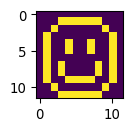
Seaborn plotting (can be skipped)
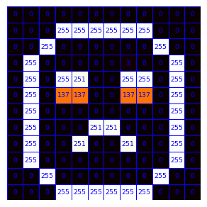
# Let's use seaborn to create some more sophisticated plots
import seaborn as sns
def mw_showimg2(img, annotcolor='white',SX=8,SY=8,SF=7,VMIN=0,VMAX=255, CMAP='hot', FMT="d"):
fig, ax = plt.subplots(1,1, figsize=(SX/2.54, SY/2.54))
_ = sns.heatmap(img, annot=True,
fmt=FMT,
cmap=CMAP,
annot_kws={"size": SF, "color": annotcolor},
vmin=VMIN, vmax=VMAX,
linewidths=.5, linecolor=annotcolor,
ax=ax)
ax.axis('off')
ax.collections[0].colorbar.remove()
plt.tight_layout()
# Plot the images
mw_showimg2(img_happy, annotcolor='blue')
mw_showimg2(img_sad2, annotcolor='blue')
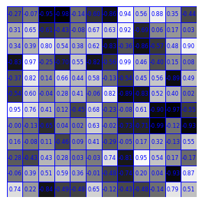
# Plot some made-up weights
img_randomweights = np.random.uniform(-1, 1, (12, 12))
mw_showimg2(img_randomweights, annotcolor='blue', SF=6,VMIN=-1,VMAX=1.0, FMT=".2f", CMAP='gray')
# Plot some made-up output
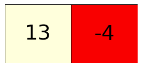
mw_showimg2(np.array([[13,-4]]), annotcolor='black', SY=4, SF=32,VMIN=-14,VMAX=14,CMAP='hot')# gray
Math (can be skipped)
For a prediction y_j, where j is referring to the categories that need predicting (e.g. \(y_1\) high means a “happy” emoji, and a high \(y_2\) value indicates the emoji is likely “sad”), \(y_j\) values can be calculated from the \(i\text{th}\) image pixel \(x_i\) as follows (with \(w_{i,j}\) being the weights):
\(\huge y_j = \sum_{i} w_{i,j} * x_i\)
Defining a data loader
To train a model, pytorch needs to be able to quickly look at a load of data efficiently. In the pytorch workflow, a data class is defined, such that training data can be stored in tensor format, and can be supplied easily to the training algorithm later.
class Data_HappySad(Dataset):
    # Again, we use a class, see above for an explanation.
    # (Remember the blueprint/house analogy.)
    #
    # This class is based on the pytorch "Dataset" class, defined
    # in the pytorch library. Data_HappySad is the name we
    # give to this class. Hence the notation "Data_HappySad(Dataset)".

    def __init__(self, targetdevice=DEVICE):

        # Technical: tell the class how to store the data (e.g. on CPU or GPU)
        self.targetdevice = targetdevice

        # Data can be handled in many ways.
        # Here, we'll store some data in the object directly.
        # This can be done by the "self." command, which refers
        # to the to-be-created object itself.
        #
        # The data needs to be converted to tensor for later use
        # We'll use the images loaded earlier, and store 3 images here
        self.data   = torch.tensor([img_happy, img_sad, img_sad2],
                                   dtype=torch.float32)

        # Now, we supply also the true labels that need to be learned
        self.label  = torch.tensor([0        , 1,       1],
                                   dtype=torch.long)

        # Technical: normalize the images
        self.data = self.data / 255.0

    def __len__(self):
        # Function required by pytorch; tells how many samples are in the dataset

        return len(self.data)

    def __getitem__(self, idx):
        # Function required by pytorch; tells how to get a specific item

        return self.data[idx].to(self.targetdevice), self.label[idx].to(self.targetdevice)
# Show an image from the dataloader
# Create an object from the class
data_happysad = Data_HappySad()
# We can extract a sample and annotation from that class
# (This will later be done automatically in the training loop)
img, label = data_happysad[0]
# For now, let's convert it to the numpy format for illustration
# purposes
img_np = img.cpu().numpy()
# Plot it
mw_showimg2(img_np, annotcolor='blue', VMIN=0, VMAX=1.0, FMT=".2f", SX=5, SY=5, SF=4)/var/folders/8w/2thz_cgn3xn13rhrxb2dvb5w0000gn/T/ipykernel_73118/2723620338.py:21: UserWarning:
Creating a tensor from a list of numpy.ndarrays is extremely slow. Please consider converting the list to a single numpy.ndarray with numpy.array() before converting to a tensor. (Triggered internally at /Users/runner/miniforge3/conda-bld/libtorch_1741947704867/work/torch/csrc/utils/tensor_new.cpp:257.)
Exercise
- Edit the code above, specifically the subfunction
__init__, such that it will load the images you created earlier at the start of this notebook. - Execute the code in the cell directly above, to check if you can make it show your own image.
- This code will show the first image in your dataset, can you also make it show the 2nd and 3rd image?
Concise answers
- To load your own images, replace the
self.dataandself.labelappropriately. - To show different images, change the index in
data_happysad[0]to another number.
Dataloader
We’re now getting close to actually training this model. We’ll need to define a dataloader. In more advanced neural network setups, the DataLoader provides convenient functionalities like shuffling the data, or loading it in parallel from disk. Here, we’ll just use it to be able to loop over the data easily, and provide the data in batches of three images.
We’ll also initialize the model itself (create an object from the class VerySimpleNN defined earlier).
# initialize the dataset and dataloader objects
my_data_happysad = Data_HappySad()
my_data_happysad_loader = torch.utils.data.DataLoader(my_data_happysad,
                                                      batch_size=3, shuffle=False)

# initialize the model
my_simple_model  = VerySimpleNN().to(DEVICE)
# Let's check the data object works as expected
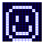
my_data_happysad.__getitem__(0)(tensor([[0., 0., 0., 0., 0., 0., 0., 0., 0., 0., 0., 0.],
[0., 0., 0., 1., 1., 1., 1., 1., 1., 0., 0., 0.],
[0., 0., 1., 0., 0., 0., 0., 0., 0., 1., 0., 0.],
[0., 1., 0., 0., 0., 0., 0., 0., 0., 0., 1., 0.],
[0., 1., 0., 0., 1., 0., 0., 1., 0., 0., 1., 0.],
[0., 1., 0., 0., 1., 0., 0., 1., 0., 0., 1., 0.],
[0., 1., 0., 0., 0., 0., 0., 0., 0., 0., 1., 0.],
[0., 1., 0., 1., 0., 0., 0., 0., 1., 0., 1., 0.],
[0., 1., 0., 1., 0., 0., 0., 0., 1., 0., 1., 0.],
[0., 1., 0., 0., 1., 1., 1., 1., 0., 0., 1., 0.],
[0., 0., 1., 0., 0., 0., 0., 0., 0., 1., 0., 0.],
[0., 0., 0., 1., 1., 1., 1., 1., 1., 0., 0., 0.]], device='mps:0'),
tensor(0, device='mps:0'))Question
- The amount of classes and library functions used at this point might be a bit overwhelming. Can you draw a cartoon that depicts the fundamental aspects of the workflow (or otherwise recreate an overview of it)?
Concise answers
- (..)
The actual training
Now we need to train the model by presenting it a picture, calculating the prediction (which might be completely off initially), determine which weight adjustments would improve the prediction (using the loss function), and update the weights accordingly. And repeat that multiple times.
Training a “real” neural network might take presenting the model with many images, for many iterations, and might take hours or days.
Here, our extremely simple model will be trained swiftly.
# Create the training loop

# Define a loss function
# This function is defined such that it will have a high value
# if there is a large discrepancy between the predicted and true labels.
# Our aim is to minimize the observed loss during the training.
loss_fn = torch.nn.CrossEntropyLoss()
# Later, we'll determine in which directions to adjust the weights
# (called the gradient), that correspond to a reduction in the loss,
# the optimizer will be used to update (optimize) the weights accordingly.
optimizer = torch.optim.Adam(my_simple_model.parameters(), lr=.01)

# technical; set model to training mode
my_simple_model.train()

# For illustratory purposes, we'll track what happens with the
# gradients and weights during the training. In a more extensive
# model, this isn't possible, as this will be too much data.
gradient_list = [] # only for illustratory purposes
weight_list   = [] # only for illustratory purposes
loss_list     = []
# Now train for 300 iterations (called epochs when 1 iteration covers all data)
for epoch_idx in range(300):

    # This loop is a bit redundant here, since we have only 3 images,
    # in a usual scenario, e.g. with 60.000 images, you would loop
    # over those images in multiple batches. Here, we'll only
    # have 1 batch, containing three images, so this loop will
    # just iterate once.
    for b_idx, (X,y) in enumerate(my_data_happysad_loader):

        # X will contain a batch of images
        # y will contain the corresponding labels

        # For illustrative purposes, we'll track the weights in the model
        # This isn't part of a usual training loop.
        weights = my_simple_model.linear.weight.detach().cpu().numpy()
        weight_list.append(weights)

        # Now determine the prediction for X based on current weights
        # (Note: the weights are stored inside the model object)
        # (Note: the model is programmed such that it will predict
        # for multiple images at once.)
        pred = my_simple_model(X)

        # Now we'll calculate the loss, or the discrepancy between
        # the predicted and true labels
        loss = loss_fn(pred, y)

        # And based on that calculation, we'll determine the gradients
        # (ie directions in which to adjust the weights to reduce the loss)
        loss.backward()

        # For illustrative purposes, we'll track the gradients
        # This wouldn't be done in a usual training loop.
        gradients = my_simple_model.linear.weight.grad.detach().cpu().numpy()
        gradient_list.append(gradients)
        # Similarly, also save the loss, this is actually also sometimes
        # monitored during "real" training scenarios.
        loss_list.append(loss.item())

        # Then we use the optimizer to apply the gradients
        optimizer.step()
        # And we reset them before the next iteration
        optimizer.zero_grad()

        # Print some information to see what's going on
        print('epoch =', epoch_idx, 'batch =',b_idx,', loss = ', loss.item())#, 'X.shape=', X.shape)
epoch = 0 batch = 0 , loss = 0.6523615717887878
epoch = 1 batch = 0 , loss = 0.6355621814727783
epoch = 2 batch = 0 , loss = 0.555995762348175
epoch = 3 batch = 0 , loss = 0.5293073654174805
epoch = 4 batch = 0 , loss = 0.4972018003463745
epoch = 5 batch = 0 , loss = 0.4491978883743286
epoch = 6 batch = 0 , loss = 0.40848013758659363
epoch = 7 batch = 0 , loss = 0.38166046142578125
epoch = 8 batch = 0 , loss = 0.3598231375217438
epoch = 9 batch = 0 , loss = 0.3348260223865509
epoch = 10 batch = 0 , loss = 0.3076183497905731
epoch = 11 batch = 0 , loss = 0.28324440121650696
epoch = 12 batch = 0 , loss = 0.2645033299922943
epoch = 13 batch = 0 , loss = 0.24978935718536377
epoch = 14 batch = 0 , loss = 0.2356160432100296
epoch = 15 batch = 0 , loss = 0.22029368579387665
epoch = 16 batch = 0 , loss = 0.2046922892332077
epoch = 17 batch = 0 , loss = 0.19055970013141632
epoch = 18 batch = 0 , loss = 0.17882661521434784
epoch = 19 batch = 0 , loss = 0.16910617053508759
epoch = 20 batch = 0 , loss = 0.16030286252498627
epoch = 21 batch = 0 , loss = 0.15155437588691711
epoch = 22 batch = 0 , loss = 0.1427207738161087
epoch = 23 batch = 0 , loss = 0.13422036170959473
epoch = 24 batch = 0 , loss = 0.12655021250247955
epoch = 25 batch = 0 , loss = 0.11991152912378311
epoch = 26 batch = 0 , loss = 0.11413756012916565
epoch = 27 batch = 0 , loss = 0.10887102037668228
epoch = 28 batch = 0 , loss = 0.10380655527114868
epoch = 29 batch = 0 , loss = 0.09883305430412292
epoch = 30 batch = 0 , loss = 0.09402356296777725
epoch = 31 batch = 0 , loss = 0.08952665328979492
epoch = 32 batch = 0 , loss = 0.08545118570327759
epoch = 33 batch = 0 , loss = 0.08180796355009079
epoch = 34 batch = 0 , loss = 0.07851909846067429
epoch = 35 batch = 0 , loss = 0.0754702165722847
epoch = 36 batch = 0 , loss = 0.0725669413805008
epoch = 37 batch = 0 , loss = 0.06976619362831116
epoch = 38 batch = 0 , loss = 0.06707537919282913
epoch = 39 batch = 0 , loss = 0.06452899426221848
epoch = 40 batch = 0 , loss = 0.0621594600379467
epoch = 41 batch = 0 , loss = 0.05997839197516441
epoch = 42 batch = 0 , loss = 0.05797182396054268
epoch = 43 batch = 0 , loss = 0.05610834062099457
epoch = 44 batch = 0 , loss = 0.05435289070010185
epoch = 45 batch = 0 , loss = 0.05267825350165367
epoch = 46 batch = 0 , loss = 0.05107099935412407
epoch = 47 batch = 0 , loss = 0.049530547112226486
epoch = 48 batch = 0 , loss = 0.04806337133049965
epoch = 49 batch = 0 , loss = 0.04667671397328377
epoch = 50 batch = 0 , loss = 0.04537329450249672
epoch = 51 batch = 0 , loss = 0.04414963722229004
epoch = 52 batch = 0 , loss = 0.042997222393751144
epoch = 53 batch = 0 , loss = 0.041904959827661514
epoch = 54 batch = 0 , loss = 0.0408625565469265
epoch = 55 batch = 0 , loss = 0.0398625023663044
epoch = 56 batch = 0 , loss = 0.03890100494027138
epoch = 57 batch = 0 , loss = 0.0379771925508976
epoch = 58 batch = 0 , loss = 0.037091705948114395
epoch = 59 batch = 0 , loss = 0.0362454354763031
epoch = 60 batch = 0 , loss = 0.03543831408023834
epoch = 61 batch = 0 , loss = 0.034668516367673874
epoch = 62 batch = 0 , loss = 0.03393329307436943
epoch = 63 batch = 0 , loss = 0.03322900831699371
epoch = 64 batch = 0 , loss = 0.03255216404795647
epoch = 65 batch = 0 , loss = 0.03189990296959877
epoch = 66 batch = 0 , loss = 0.03127017617225647
epoch = 67 batch = 0 , loss = 0.03066176176071167
epoch = 68 batch = 0 , loss = 0.03007415495812893
epoch = 69 batch = 0 , loss = 0.029507145285606384
epoch = 70 batch = 0 , loss = 0.02896036207675934
epoch = 71 batch = 0 , loss = 0.028433119878172874
epoch = 72 batch = 0 , loss = 0.02792471833527088
epoch = 73 batch = 0 , loss = 0.02743382751941681
epoch = 74 batch = 0 , loss = 0.026959320530295372
epoch = 75 batch = 0 , loss = 0.026499846950173378
epoch = 76 batch = 0 , loss = 0.02605440653860569
epoch = 77 batch = 0 , loss = 0.025622108951210976
epoch = 78 batch = 0 , loss = 0.025202354416251183
epoch = 79 batch = 0 , loss = 0.02479471266269684
epoch = 80 batch = 0 , loss = 0.02439872734248638
epoch = 81 batch = 0 , loss = 0.02401428483426571
epoch = 82 batch = 0 , loss = 0.02364088036119938
epoch = 83 batch = 0 , loss = 0.023278215900063515
epoch = 84 batch = 0 , loss = 0.022925645112991333
epoch = 85 batch = 0 , loss = 0.022582797333598137
epoch = 86 batch = 0 , loss = 0.02224910818040371
epoch = 87 batch = 0 , loss = 0.021924206987023354
epoch = 88 batch = 0 , loss = 0.02160753309726715
epoch = 89 batch = 0 , loss = 0.02129875309765339
epoch = 90 batch = 0 , loss = 0.020997652783989906
epoch = 91 batch = 0 , loss = 0.02070397138595581
epoch = 92 batch = 0 , loss = 0.020417412742972374
epoch = 93 batch = 0 , loss = 0.020137719810009003
epoch = 94 batch = 0 , loss = 0.019864829257130623
epoch = 95 batch = 0 , loss = 0.01959844119846821
epoch = 96 batch = 0 , loss = 0.019338222220540047
epoch = 97 batch = 0 , loss = 0.019084064289927483
epoch = 98 batch = 0 , loss = 0.018835701048374176
epoch = 99 batch = 0 , loss = 0.018592914566397667
epoch = 100 batch = 0 , loss = 0.0183554757386446
epoch = 101 batch = 0 , loss = 0.018123194575309753
epoch = 102 batch = 0 , loss = 0.01789592206478119
epoch = 103 batch = 0 , loss = 0.01767350360751152
epoch = 104 batch = 0 , loss = 0.01745578832924366
epoch = 105 batch = 0 , loss = 0.01724262535572052
epoch = 106 batch = 0 , loss = 0.017033936455845833
epoch = 107 batch = 0 , loss = 0.01682957075536251
epoch = 108 batch = 0 , loss = 0.0166292954236269
epoch = 109 batch = 0 , loss = 0.0164331141859293
epoch = 110 batch = 0 , loss = 0.01624087616801262
epoch = 111 batch = 0 , loss = 0.016052424907684326
epoch = 112 batch = 0 , loss = 0.015867652371525764
epoch = 113 batch = 0 , loss = 0.015686480328440666
epoch = 114 batch = 0 , loss = 0.015508793294429779
epoch = 115 batch = 0 , loss = 0.015334445051848888
epoch = 116 batch = 0 , loss = 0.01516343280673027
epoch = 117 batch = 0 , loss = 0.01499564666301012
epoch = 118 batch = 0 , loss = 0.014830891974270344
epoch = 119 batch = 0 , loss = 0.014669212512671947
epoch = 120 batch = 0 , loss = 0.01451049279421568
epoch = 121 batch = 0 , loss = 0.01435465831309557
epoch = 122 batch = 0 , loss = 0.014201556332409382
epoch = 123 batch = 0 , loss = 0.01405122596770525
epoch = 124 batch = 0 , loss = 0.01390355359762907
epoch = 125 batch = 0 , loss = 0.013758542947471142
epoch = 126 batch = 0 , loss = 0.013615995645523071
epoch = 127 batch = 0 , loss = 0.013475877232849598
epoch = 128 batch = 0 , loss = 0.013338190503418446
epoch = 129 batch = 0 , loss = 0.013202817179262638
epoch = 130 batch = 0 , loss = 0.013069760985672474
epoch = 131 batch = 0 , loss = 0.012938941828906536
epoch = 132 batch = 0 , loss = 0.012810245156288147
epoch = 133 batch = 0 , loss = 0.01268371194601059
epoch = 134 batch = 0 , loss = 0.012559263966977596
epoch = 135 batch = 0 , loss = 0.01243678480386734
epoch = 136 batch = 0 , loss = 0.012316353619098663
epoch = 137 batch = 0 , loss = 0.01219781581312418
epoch = 138 batch = 0 , loss = 0.01208117138594389
epoch = 139 batch = 0 , loss = 0.011966384015977383
epoch = 140 batch = 0 , loss = 0.011853412725031376
epoch = 141 batch = 0 , loss = 0.011742182075977325
epoch = 142 batch = 0 , loss = 0.011632693000137806
epoch = 143 batch = 0 , loss = 0.011524907313287258
epoch = 144 batch = 0 , loss = 0.01141874585300684
epoch = 145 batch = 0 , loss = 0.01131421234458685
epoch = 146 batch = 0 , loss = 0.01121122669428587
epoch = 147 batch = 0 , loss = 0.011109829880297184
epoch = 148 batch = 0 , loss = 0.011009983718395233
epoch = 149 batch = 0 , loss = 0.01091157179325819
epoch = 150 batch = 0 , loss = 0.01081459317356348
epoch = 151 batch = 0 , loss = 0.010719050653278828
epoch = 152 batch = 0 , loss = 0.010624904185533524
epoch = 153 batch = 0 , loss = 0.010532155632972717
epoch = 154 batch = 0 , loss = 0.010440685786306858
epoch = 155 batch = 0 , loss = 0.010350576601922512
epoch = 156 batch = 0 , loss = 0.010261707939207554
epoch = 157 batch = 0 , loss = 0.010174122639000416
epoch = 158 batch = 0 , loss = 0.010087779723107815
epoch = 159 batch = 0 , loss = 0.010002600960433483
epoch = 160 batch = 0 , loss = 0.009918666444718838
epoch = 161 batch = 0 , loss = 0.009835819713771343
epoch = 162 batch = 0 , loss = 0.009754178114235401
epoch = 163 batch = 0 , loss = 0.009673585183918476
epoch = 164 batch = 0 , loss = 0.009594121016561985
epoch = 165 batch = 0 , loss = 0.009515783749520779
epoch = 166 batch = 0 , loss = 0.00943841878324747
epoch = 167 batch = 0 , loss = 0.009362143464386463
epoch = 168 batch = 0 , loss = 0.009286840446293354
epoch = 169 batch = 0 , loss = 0.009212548844516277
epoch = 170 batch = 0 , loss = 0.009139190427958965
epoch = 171 batch = 0 , loss = 0.009066884405910969
epoch = 172 batch = 0 , loss = 0.008995474316179752
epoch = 173 batch = 0 , loss = 0.0089249974116683
epoch = 174 batch = 0 , loss = 0.008855416439473629
epoch = 175 batch = 0 , loss = 0.008786731399595737
epoch = 176 batch = 0 , loss = 0.008718864060938358
epoch = 177 batch = 0 , loss = 0.008651932701468468
epoch = 178 batch = 0 , loss = 0.00858581904321909
epoch = 179 batch = 0 , loss = 0.008520563133060932
epoch = 180 batch = 0 , loss = 0.008456086739897728
epoch = 181 batch = 0 , loss = 0.008392429910600185
epoch = 182 batch = 0 , loss = 0.008329511620104313
epoch = 183 batch = 0 , loss = 0.008267414756119251
epoch = 184 batch = 0 , loss = 0.008206096477806568
epoch = 185 batch = 0 , loss = 0.008145480416715145
epoch = 186 batch = 0 , loss = 0.008085567504167557
epoch = 187 batch = 0 , loss = 0.008026473224163055
epoch = 188 batch = 0 , loss = 0.007968042977154255
epoch = 189 batch = 0 , loss = 0.00791027583181858
epoch = 190 batch = 0 , loss = 0.007853210903704166
epoch = 191 batch = 0 , loss = 0.0077968500554561615
epoch = 192 batch = 0 , loss = 0.007741112262010574
epoch = 193 batch = 0 , loss = 0.0076860785484313965
epoch = 194 batch = 0 , loss = 0.007631629705429077
epoch = 195 batch = 0 , loss = 0.007577845361083746
epoch = 196 batch = 0 , loss = 0.007524725515395403
epoch = 197 batch = 0 , loss = 0.007472152356058359
epoch = 198 batch = 0 , loss = 0.00742020457983017
epoch = 199 batch = 0 , loss = 0.007368803024291992
epoch = 200 batch = 0 , loss = 0.007318027317523956
epoch = 201 batch = 0 , loss = 0.007267799228429794
epoch = 202 batch = 0 , loss = 0.007218156475573778
epoch = 203 batch = 0 , loss = 0.0071691409684717655
epoch = 204 batch = 0 , loss = 0.007120514754205942
epoch = 205 batch = 0 , loss = 0.007072554435580969
epoch = 206 batch = 0 , loss = 0.007025022525340319
epoch = 207 batch = 0 , loss = 0.006978078279644251
epoch = 208 batch = 0 , loss = 0.006931682582944632
epoch = 209 batch = 0 , loss = 0.00688571622595191
epoch = 210 batch = 0 , loss = 0.006840298417955637
epoch = 211 batch = 0 , loss = 0.0067953490652143955
epoch = 212 batch = 0 , loss = 0.006750870496034622
epoch = 213 batch = 0 , loss = 0.006706899497658014
epoch = 214 batch = 0 , loss = 0.006663359701633453
epoch = 215 batch = 0 , loss = 0.006620329339057207
epoch = 216 batch = 0 , loss = 0.006577728781849146
epoch = 217 batch = 0 , loss = 0.006535558495670557
epoch = 218 batch = 0 , loss = 0.006493859458714724
epoch = 219 batch = 0 , loss = 0.00645251153036952
epoch = 220 batch = 0 , loss = 0.006411673501133919
epoch = 221 batch = 0 , loss = 0.006371305789798498
epoch = 222 batch = 0 , loss = 0.006331250071525574
epoch = 223 batch = 0 , loss = 0.006291665602475405
epoch = 224 batch = 0 , loss = 0.006252432707697153
epoch = 225 batch = 0 , loss = 0.006213671062141657
epoch = 226 batch = 0 , loss = 0.00617526238784194
epoch = 227 batch = 0 , loss = 0.00613720528781414
epoch = 228 batch = 0 , loss = 0.006099618971347809
epoch = 229 batch = 0 , loss = 0.006062306463718414
epoch = 230 batch = 0 , loss = 0.006025465205311775
epoch = 231 batch = 0 , loss = 0.005988936871290207
epoch = 232 batch = 0 , loss = 0.005952761974185705
epoch = 233 batch = 0 , loss = 0.005916978698223829
epoch = 234 batch = 0 , loss = 0.005881509277969599
epoch = 235 batch = 0 , loss = 0.005846431944519281
epoch = 236 batch = 0 , loss = 0.005811627954244614
epoch = 237 batch = 0 , loss = 0.005777257028967142
epoch = 238 batch = 0 , loss = 0.005743121262639761
epoch = 239 batch = 0 , loss = 0.005709377583116293
epoch = 240 batch = 0 , loss = 0.005675868596881628
epoch = 241 batch = 0 , loss = 0.005642792675644159
epoch = 242 batch = 0 , loss = 0.0056099905632436275
epoch = 243 batch = 0 , loss = 0.005577500909566879
epoch = 244 batch = 0 , loss = 0.005545287858694792
epoch = 245 batch = 0 , loss = 0.005513427313417196
epoch = 246 batch = 0 , loss = 0.005481801927089691
epoch = 247 batch = 0 , loss = 0.00545053044334054
epoch = 248 batch = 0 , loss = 0.005419494118541479
epoch = 249 batch = 0 , loss = 0.005388771649450064
epoch = 250 batch = 0 , loss = 0.005358363967388868
epoch = 251 batch = 0 , loss = 0.005328190978616476
epoch = 252 batch = 0 , loss = 0.005298332776874304
epoch = 253 batch = 0 , loss = 0.005268709268420935
epoch = 254 batch = 0 , loss = 0.005239440128207207
epoch = 255 batch = 0 , loss = 0.005210327450186014
epoch = 256 batch = 0 , loss = 0.005181529093533754
epoch = 257 batch = 0 , loss = 0.005153006408363581
epoch = 258 batch = 0 , loss = 0.00512471841648221
epoch = 259 batch = 0 , loss = 0.005096666514873505
epoch = 260 batch = 0 , loss = 0.005068889353424311
epoch = 261 batch = 0 , loss = 0.005041348282247782
epoch = 262 batch = 0 , loss = 0.005014042370021343
epoch = 263 batch = 0 , loss = 0.004987012129276991
epoch = 264 batch = 0 , loss = 0.004960138816386461
epoch = 265 batch = 0 , loss = 0.004933579359203577
epoch = 266 batch = 0 , loss = 0.004907256457954645
epoch = 267 batch = 0 , loss = 0.004881130065768957
epoch = 268 batch = 0 , loss = 0.004855199251323938
epoch = 269 batch = 0 , loss = 0.004829504992812872
epoch = 270 batch = 0 , loss = 0.004804085940122604
epoch = 271 batch = 0 , loss = 0.004778823349624872
epoch = 272 batch = 0 , loss = 0.0047538368962705135
epoch = 273 batch = 0 , loss = 0.004729007370769978
epoch = 274 batch = 0 , loss = 0.004704413469880819
epoch = 275 batch = 0 , loss = 0.004680016543716192
epoch = 276 batch = 0 , loss = 0.004655855242162943
epoch = 277 batch = 0 , loss = 0.0046318513341248035
epoch = 278 batch = 0 , loss = 0.004608083516359329
epoch = 279 batch = 0 , loss = 0.004584512207657099
epoch = 280 batch = 0 , loss = 0.0045611378736793995
epoch = 281 batch = 0 , loss = 0.004537920001894236
epoch = 282 batch = 0 , loss = 0.004514938686043024
epoch = 283 batch = 0 , loss = 0.004492154344916344
epoch = 284 batch = 0 , loss = 0.004469527397304773
epoch = 285 batch = 0 , loss = 0.0044470964930951595
epoch = 286 batch = 0 , loss = 0.004424822982400656
epoch = 287 batch = 0 , loss = 0.004402706865221262
epoch = 288 batch = 0 , loss = 0.0043808273039758205
epoch = 289 batch = 0 , loss = 0.004359144251793623
epoch = 290 batch = 0 , loss = 0.004337579011917114
epoch = 291 batch = 0 , loss = 0.004316210746765137
epoch = 292 batch = 0 , loss = 0.004294999409466982
epoch = 293 batch = 0 , loss = 0.004273945931345224
epoch = 294 batch = 0 , loss = 0.004253089427947998
epoch = 295 batch = 0 , loss = 0.004232389852404594
epoch = 296 batch = 0 , loss = 0.004211848136037588
epoch = 297 batch = 0 , loss = 0.004191463813185692
epoch = 298 batch = 0 , loss = 0.004171276465058327
epoch = 299 batch = 0 , loss = 0.004151206463575363Questions
- Above you see a training loop, in the printed output below:
- Why is the loss decreasing?
- Optional: google what “learning rate” means. This is set by the
lrparameter. If you like, you can re-initialize the model, adjustlrin the cell above, and see what the effect is. - What would happen to the loss if you’d train for more iterations?
- Would you reckon the training has worked? Will the model now recognize something?
Concise answers
- The loss is decreasing since the training is working: a gradient is calculated that shows in which direction each weight should be adjusted to lower the loss. And indeed, this is done each iteration, such that the loss decreases.
- Regarding learning rate; the gradient only gives the direction in which to adjust the weights (how the weights should be adjusted relative to each other), but not by how much. The learning rate scales to what extend the weights are adjusted. If the learning rate is too high, you might “overshoot” the optimal weights, and end up with a higher loss again. If it’s too low, training will be very slow.
- If you train for more iterations, the loss will likely decrease further.
- For the original examples, the trianing has likely worked, as the loss decreased a load. However, since the model is so simple, and the training data is so limited, it probably won’t be able to recognize anything beyond these specific images.
Loss value over time
# Let's plot the loss value over time
_ = plt.plot(np.array(loss_list).squeeze())
plt.xlabel('Iteration (or epoch)'); plt.ylabel('Loss value')
Text(0, 0.5, 'Loss value')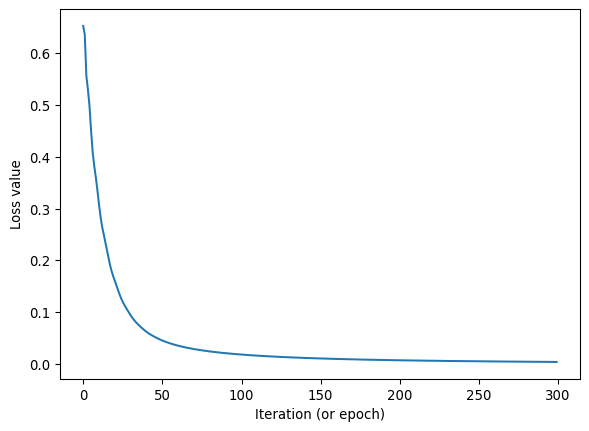
Visualization of what happened
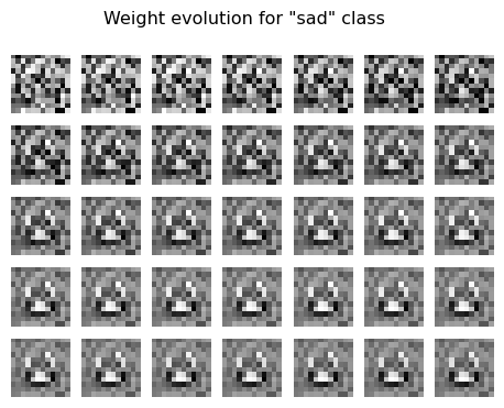
The code below visualizes what happened during model training with the weights. Since this model is so simple, we can interpret the weights.
# visualize the weights
TO_SHOW_NR = 35
fig, axs = plt.subplots(TO_SHOW_NR//7, 7, figsize=(15/2.54, 15/2.54*(TO_SHOW_NR//7)/7))
# show the weights of weight_list[X][0] in a 5 x 7 grid
for weight_iteration in range(TO_SHOW_NR):
    pos_X = weight_iteration//7
    pos_Y = weight_iteration%7
    _ = axs[pos_X,pos_Y].imshow(weight_list[weight_iteration][0].reshape(12,12), cmap='gray')
    _ = axs[pos_X,pos_Y].axis('off')
plt.suptitle('Weight evolution for "happy" class')

# now the same for the "sad" class
fig, axs = plt.subplots(TO_SHOW_NR//7, 7, figsize=(15/2.54, 15/2.54*(TO_SHOW_NR//7)/7))
# show the weights of weight_list[X][1] in a 5 x 7 grid
for weight_iteration in range(TO_SHOW_NR):
    pos_X = weight_iteration//7
    pos_Y = weight_iteration%7
    _ = axs[pos_X,pos_Y].imshow(weight_list[weight_iteration][1].reshape(12,12), cmap='gray')
    _ = axs[pos_X,pos_Y].axis('off')
plt.suptitle('Weight evolution for "sad" class')
Text(0.5, 0.98, 'Weight evolution for "sad" class')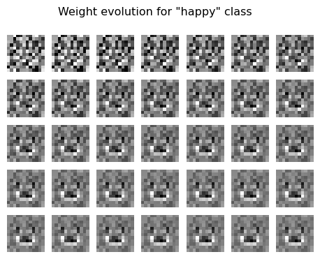
Questions
- Update the code
plt.suptitles above to reflect the categories that match the labels for the images you created yourself. - Right to left, top to bottom, we see how the weights are updated over multiple iterations. Why do you think the weights change the way they do?
- Do you recognize any features in it from your input images?
# show the final weights as images
fig, axs = plt.subplots(1,2, figsize=(8/2.54, 4/2.54))
_=axs[0].imshow(weight_list[-1][0].reshape(12,12),cmap='gray')
_=axs[1].imshow(weight_list[-1][1].reshape(12,12),cmap='gray')
_=axs[0].set_title('happy')
_=axs[1].set_title('sad')
_=axs[0].axis('off')
_=axs[1].axis('off')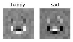
Questions
- Update the labels above according with your own data.
- How do you think this model would perform on a validation data set (as opposed to a training set)?
- Do you think overfitting is a problem for this model?
- In a more complex network architecture, do you think it will be possible to interpret weights in the same way as we did here?
Concise answers
- (..)
- This model will likely perform very poorly on a validation set, since it is overfitted on the few training images it saw. To detect generalized patterns, a more complex model and more training data would be needed.
- So yes, overfitting is a problem. One can test for overfitting by carefully checking performance on a validation set (pictures the model hasn’t seen yet), which should be good if the model is not overfitted.
- In a more complex network architecture, it will likely not be possible to interpret the weights in the same way as we did here, since there are many more parameters, and they interact in a more complex way. There are ways to try to interpret the results of complex models, but this is wholly outside our scope, and it is not always possible to fully understand how a complex model makes its decisions.
Proof of the pudding: did it work?
Let’s feed the original input images to the model again, and look at the predictions. (In a real scenario, you’d hope the model will also be able to classify unseen data, with our limited training data and limited model, that’s not something we can expect.)
# apply the model to image 1
X1 = my_data_happysad.__getitem__(0)[0].unsqueeze(0)
pred = my_simple_model(X1)
print('X1=', pred)
# and to image 2
X2 = my_data_happysad.__getitem__(1)[0].unsqueeze(0)
pred = my_simple_model(X2)
print('X2=', pred)
# and to image 3
X3 = my_data_happysad.__getitem__(2)[0].unsqueeze(0)
pred = my_simple_model(X3)
print('X3=', pred)
X1= tensor([[ 2.5303, -2.5606]], device='mps:0', grad_fn=<LinearBackward0>)
X2= tensor([[-2.6224, 2.5316]], device='mps:0', grad_fn=<LinearBackward0>)
X3= tensor([[-3.8946, 3.7043]], device='mps:0', grad_fn=<LinearBackward0>)Questions
- Are the predictions correct?
- Try drawing a new image in one of your classes, and let the model predict the class. What do you see?
Concise answers
- If the location in the array corresponding to the actual class has the highest value, then the prediction is correct.
- If your old and new images have specific pixels that consistently show different values per class, it might be that the class gets predicted correctly, as this simple model will pick up on those. But as mentioned throughout earlier answers, this model is very simple, and the training data is very limited, so it won’t be able to generalize well to new images.
Biological images
- Say you have biological data from multiple conditions and multiple biological replicates. How would you divide this data among the training and validation sets?
- Let’s say you use an existing machine learning model (e.g. micro-sam) to segment your data. Do you think you can manually check the segmentation went OK by investigating the original input images and segmentation result?
- Now, let’s say you use a machine learning model to quantify a specific phenotype (say ‘leaf health’ trained on human scoring of leafs) that you expect to change for your conditions.
- Is it now equally easy as the previous question to check whether the score correctly reflects leaf health?
- If you use a more complex machine learning model, is it possible to understand how the scoring was determined, or which features the model used to make its decision? What challenges might arise in interpreting the results?
- Is the interpretability equally important for segmentation and for phenotyping?
- What are your thoughts on applying ML in this way?
- Say the images used to train the leaf damage also included (in the picture) several groups of insects that contribute to the damage in various degree respectively. Do you see any issue with this training data set?
- How could overfitting impact the performance of your model when applied to new biological images?
- How might differences in image acquisition (e.g. microscope settings, lighting) influence the results of your analysis?
- How can you assess whether your model is generalizing well to unseen data, rather than just memorizing the training set?
Concise answers
My thoughts:
- Ideally, both the training and validation class reflect the same distribution of data, so you would want to have a mix of conditions and biological replicates in both sets. You could for example randomly assign 80% of the data to the training set, and 20% to the validation set, while ensuring that all conditions and replicates are represented in both sets.
- Generally, it’s easy to see by eye, even in new images, whether segmentation corresponds to the intended result. Manually drawing segmentations is likely much more work than quickly checking whether the segmentation is correct.
- Phenotype learning:
- It’s not as easy to check whether the score correctly reflects leaf health, since this is a more abstract concept than segmentation. Manually checking all output will likely be difficult, as this is almost as laborious as checking predicted scores.
- It will be very hard to understand how the model determined its score, in case you have used a more complex model. The model is a “black box”.
- Segmentation usually either has worked or not. How something is recognized is usually not key to understanding your biological question (depending on your topic). On the other hand, understanding the phenotype, and its nuances, is probably much more related to your biological question.
- I would try to avoid “black box” approaches as solution to biological questions.
Congratulations!
You have reached the end of the machine learning part of this workshop! Let us know if you have any questions, comments or discussion points.
img_party=tiff.imread('images/emoji/party.tif')
fig, axs = plt.subplots(1,4, figsize=(12/2.54, 3/2.54))
for ch in range(3):
    _=axs.flatten()[ch].imshow(img_party[:,:,ch])
_=axs.flatten()[3].imshow(img_party)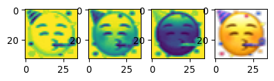
More code for other purposes (can be skipped)
# Final weights in different style
print(np.min(weight_list[-1][0]), np.max(weight_list[-1][0]))
mw_showimg2(weight_list[-1][0].reshape((12,12)),
            annotcolor='blue', VMIN=-1, VMAX=1.0, FMT=".2f", CMAP='gray', SF=6)
-0.7964875 0.69642836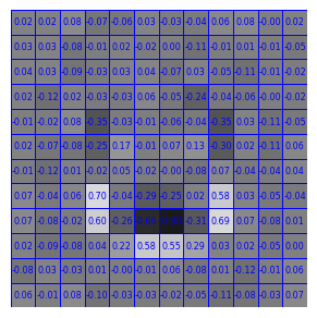
# show the first and second gradients
fig, axs = plt.subplots(2,3, figsize=(12/2.54, 6/2.54))
_=axs[0,0].imshow(gradient_list[0][0].reshape(12,12))
_=axs[0,1].imshow(gradient_list[1][0].reshape(12,12))
_=axs[0,2].imshow(gradient_list[2][0].reshape(12,12))
_=axs[1,0].imshow(gradient_list[3][0].reshape(12,12))
_=axs[1,1].imshow(gradient_list[4][0].reshape(12,12))
_=axs[1,2].imshow(gradient_list[5][0].reshape(12,12))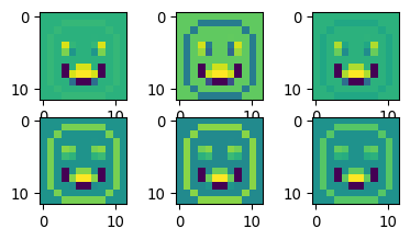
print(len(gradient_list))
gradient_list[0].shape
gradient_list[4][0].reshape((12,12)).shape300(12, 12)# Doesn't seem to work ??
# from torchsummary import summary
# summary(my_simple_model, input_size=(12,12))# There should be 12x12 + 1 + 12x12 + 1 = 290 model parameters
sum(p.numel() for p in my_simple_model.parameters() if p.requires_grad)290