# libraries
import matplotlib.pyplot as plt
import seaborn as sns
import tifffile as tiff
import numpy as np

# some new ones
import skimage as sk
from scipy import stats
from scipy import ndimageWorkshop Python Image Analysis
Martijn Wehrens, 2026-04
Estimated time: XX mins presenting + YY mins exercises
Chapter IIIA: Image Processing
Image processing entails modifying images, using mathematical operations, in order to enhance them, or to later being able to better extract information from them.
Math can be applied to images
# Load a picture of fluorescently labeled HeLa cells
img_path = 'images/biological/exampleHeLa.tif'
img_HeLa = tiff.imread(img_path)

# Image statistics
print('Mean: ',img_HeLa.mean())
print('Min: ', img_HeLa.min())
print('Max: ', img_HeLa.max())
print('Standard dev: ', img_HeLa.std())

# Now the mode and percentiles
print('Mode: ', np.bincount(img_HeLa.ravel()).argmax())
print('5th percentile: ', np.percentile(img_HeLa, 5))
print('95th percentile: ', np.percentile(img_HeLa, 95))
Mean: 430.6844697667808
Min: 324
Max: 14822
Standard dev: 277.61160166795554
Mode: 403
5th percentile: 393.0
95th percentile: 441.0# Adjust contrast
new_min = np.percentile(img_HeLa, 3)
new_max = np.percentile(img_HeLa, 95)
print([new_min, new_max])
# Changing the image values according formula
img_HeLa_norm = img_HeLa.copy()
img_HeLa_norm[img_HeLa_norm < new_min] = new_min
img_HeLa_norm[img_HeLa_norm > new_max] = new_max
img_HeLa_norm = (img_HeLa_norm - new_min)/( new_max-new_min ) * 2**16
# Plot the original once more
_ = plt.imshow(img_HeLa, cmap='viridis', vmin=0, vmax=2**16)
plt.show()
# And the normalized image
_ = plt.imshow(img_HeLa_norm, cmap='viridis', vmin=0, vmax=2**16)
plt.show()
# Only change the display
_ = plt.imshow(img_HeLa, cmap='viridis', vmin=new_min, vmax=new_max)
plt.show()
# Don't throw away your raw images!
# If you save modified images like this, create a copy.[np.float64(391.0), np.float64(441.0)]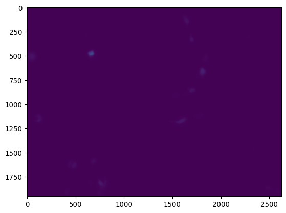

_ = plt.hist(img_HeLa_norm.ravel(), bins=256)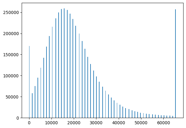
Further adjusting contrast
When looking at an image you might see striking features, and think that’s all your looking at.
However, both for humans looking at pictures, and for computers analyzing pictures, features can remain unseen depending on display or processing.
# something convenient for later
FIGSIZE21 = (10/2.54,5/2.54)
FIGSIZE22 = (10/2.54,10/2.54)
# More advanced contrast adjustment
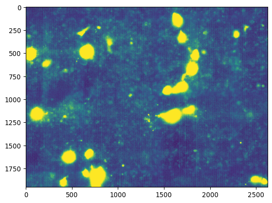
# Let's say we're investigating marine microogranism E. moji,
# and we've taken the microscopy image below.
image_path = 'images/emoji/emojis-swimming.tif'
img_emoji = tiff.imread(image_path)
# And now we're displaying the image:
_ = plt.imshow(img_emoji, cmap='grey')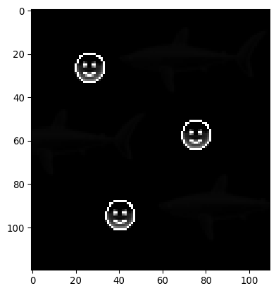
# Great! Three specimen are swimming around happily!

# But wait..
_ = plt.imshow(img_emoji, cmap='viridis')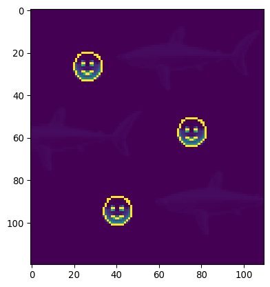
# The viridis colormap shows us there might be some more signal.

# (You can also try to open this image in FIJI, and play around with contrast.)

# There appears to be an import signal in the low range
#   "high dynamic range"

# "Nice looking" figure with contrast enhancements

fig, axs = plt.subplots(2,3)

# Apply gamma transformation
img_emoji_gamma = sk.exposure.adjust_gamma(img_emoji, gamma=0.5)
_ = axs[0,0].imshow(img_emoji_gamma)
_ = axs[0,0].set_title(f'Gamma ($\\gamma=0.5$)')
    # see also
    # https://docs.python.org/3/tutorial/inputoutput.html
    # https://matplotlib.org/stable/users/explain/text/mathtext.html

# Use a simple log
img_emoji_log = np.log(1+img_emoji/255*254)
_ = axs[0,1].imshow(img_emoji_log)
_ = axs[0,1].set_title('Log')

# Normalize the image by 20
img_emoji_norm = img_emoji.copy()
img_emoji_norm[img_emoji_norm>20] = 20
img_emoji_norm = img_emoji_norm/20*255
_ = axs[0,2].imshow(img_emoji_norm)
_ = axs[0,2].set_title('Rescaled')
#_ = axs[2].imshow(sk.exposure.adjust_gamma(img_emoji, gamma=2.0))

# Show the corresponding histograms
_ = axs[1,0].hist(img_emoji_gamma.ravel(), bins=50)
_ = axs[1,1].hist(img_emoji_log.ravel(), bins=50)
_ = axs[1,2].hist(img_emoji_norm.ravel(), bins=50)

plt.tight_layout()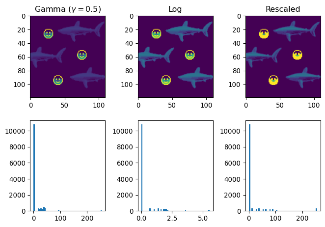
# Show the gamma input/output relation
x = np.linspace(0,255,100)
x_transformed = sk.exposure.adjust_gamma(x, gamma=0.5)
x_transformed_255 = x_transformed/np.max(x_transformed)*255

fig, ax = plt.subplots()
_ = ax.plot(x, x_transformed_255,
                label='gamma=0.5')
_ = ax.set_xlabel('Old px value')
_ = ax.set_ylabel('New px value')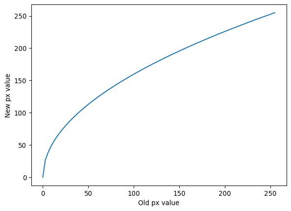
Note that these operations won’t magically put new information into the picture. But they can be really useful for visualization purposes. Especially combined with histograms.
Segmentation (1)
Segmentation is a prime example of image processing useful for biologists.
Say you want to - quantify bacterial growth, - take measurements on individual cultured cells, - or quantify leaf damage,
the computer will have to understand which pixel relates to which object (e.g. a cell) to quantify anything.
In later sections, we’ll look at how to process these annotated regions.
# Let's load some nuclei example data again
img_path_KTR = '/Users/m.wehrens/Data_notbacked/2025_Py-Image-workshop_KTR-example-data/raw/Composite_KTR.tif'
img_nuclei = tiff.imread(img_path_KTR)[0, 0, 0:200, 0:200]

fig, axs = plt.subplots(1,2, figsize=FIGSIZE21)
_ = axs[0].imshow(img_nuclei, cmap='magma')
_ = axs[1].hist(img_nuclei.ravel())
plt.tight_layout()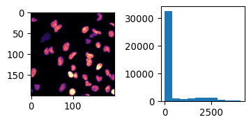
# Could we determine a manual threshold?
# .. (audience)
# yes!
mask_nuclei = img_nuclei>700
_=plt.imshow(mask_nuclei)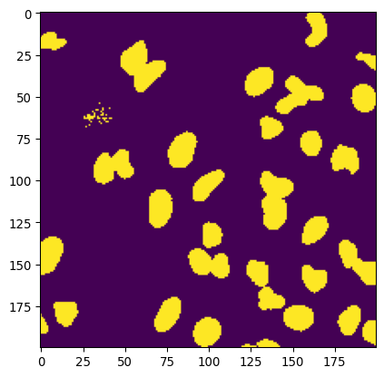
Extracting information
We’ll progress to somewhat more realistic examples later, but let’s say we want to quantify the size of the nuclei.
This requires some more tools.
# label the nuclei
labeled_nuclei = sk.measure.label(mask_nuclei)
_ = plt.imshow(labeled_nuclei)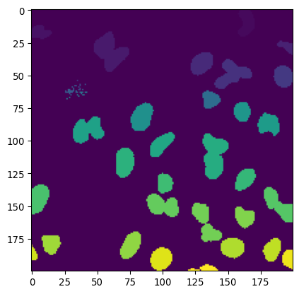
# The labeled map
# Great tool to get
#   - object properties
_ = plt.imshow(labeled_nuclei==1)
    # continuous regions of pixels
    # unique integer values

# Size 1 nucleus:
print(f"Area nuclei 1 (px): {np.sum(labeled_nuclei==1)}")
Area nuclei 1 (px): 198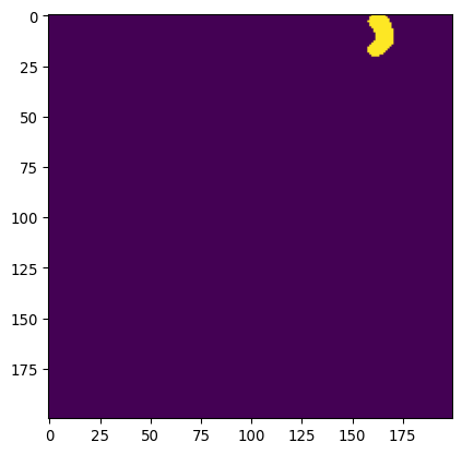
# Count all sizes
nuclei_sizes = np.array([np.sum(labeled_nuclei==label)
                         for label in range(1,np.max(labeled_nuclei))])
print(nuclei_sizes[0:10])

# and show the histogram
_ = plt.hist(nuclei_sizes)
[198 123 455 71 230 336 200 1 6 1]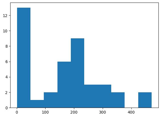
# There are functions that make such tasks much easier

# Let's get regionprops
regions = sk.measure.regionprops(labeled_nuclei, intensity_image=img_nuclei)
# Let's inspect a region object
region_1 = regions[0]
# What kind of things are stored in here?
# For more info, see:
# https://scikit-image.org/docs/0.25.x/api/skimage.measure.html#skimage.measure.regionprops
region_1.area
region_1.bbox
region_1.centroid
# And we can easily make the histogram, using:
areas = [r.area for r in regions]
_=plt.hist(areas)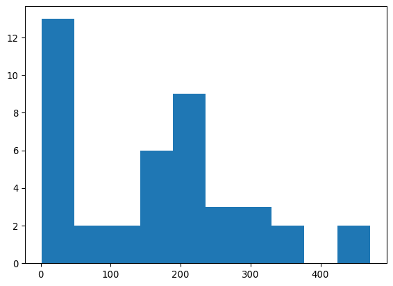
Exercises part I
E. moji
- Try to segment the “E. moji” image, both the E. mojis and the other organism (S. hark?) that are present.
- With the methods outlined earlier, this won’t be perfect.
- [Optional] You can improve your mask by “filling holes”, using the function
scipy.ndimage.binary_fill_holes(mask_emoji).
- Make a histogram of the object sizes.
- Why does the histogram look the way it looks?
Nuclei
- We made a histogram of nuclear sizes, but the sizes were in pixels. Produce a histogram with the sizes in microns. (You might need a tool like FIJI.)
- Let’s also make a more fancier plot:
- Can you also add their contours?
- And put a cross in their centers?
- [Optional] Use the functions
np.random.rand()andListedColormap()to create a colormap that’s a bit more useful to display the labeled nuclei.
Hints
Finding the scale using FIJI
Open your image in FIJI, and check out image > properties, or analyze > set scale.
Adding contours
Use the function plt.contour with a smart bins = .. setting.
Adding cross in centers
Use the .centroid property of the region to obtain points to plot as centers.
[Optional] Dodgy guys
- Load the picture
images/car/dodgy-guys.tif- Can you count the amount of dodgy guys with python?
- Can you identify where they are in the image (plot crosses on top of the image)?
- Can you annotate the sizes of each of the heads on top of their heads in a plot?
- Can you now easily identify which of the faces only occurs once in this image?