# Importing libraries

import matplotlib.pyplot as plt
    # used for plotting
import seaborn as sns
    # used for advanced plotting
import tifffile as tiff
    # used for reading images
    #
    # there are multiple libraries that can read image
    # from general purpose to science-specialized
    # other options:
    # PIL.Image.open(), imageio.imread(), skimage.io.imread() (old), ..
    #
    # tiffile is geared for scientific data;
    # handles metadata, large files, bit depth, and stacks well
    #
    # imageio is very useful to read various formats,
    # actually uses tiffile library
import numpy as np
# for general math, matrix operations, etcWorkshop Python Image Analysis
Martijn Wehrens, 2026-04
Estimated time: 30 mins presenting + 30 mins exercises
Chapter IIA: Reading, modifying and displaying images
Reading and displaying images
Setup: Importing libraries
Reading image files
# Read a tif file
image_path = 'images/emoji/emoji-8bit-gray.tif'
img = tiff.imread(image_path)

_ = plt.imshow(img)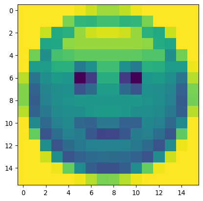
Understanding image data
_ = plt.imshow(img, cmap='gray') # we can change the display colors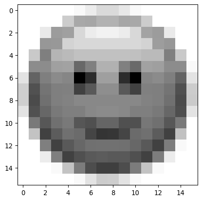
# but what is an image actually?
print(np.shape(img))
print(img)
    # (ask students)
(16, 16)
[[254 254 254 254 254 250 241 229 229 238 250 254 254 254 254 254]
[254 254 254 254 220 196 195 203 203 195 196 220 254 254 254 254]
[254 254 239 188 191 228 241 245 245 241 228 193 188 240 254 254]
[254 254 185 186 225 228 228 228 228 228 228 225 189 185 254 254]
[254 218 169 205 208 213 213 213 213 213 212 208 208 169 218 254]
[254 178 178 191 192 154 170 202 202 170 155 192 190 178 178 250]
[236 151 169 177 174 85 115 190 190 115 86 174 177 169 151 235]
[222 139 162 169 170 128 145 179 179 145 128 170 169 162 138 220]
[222 135 159 169 171 175 175 175 175 175 175 171 169 159 135 219]
[236 139 153 166 169 169 175 177 177 175 169 169 166 153 137 236]
[254 165 143 159 166 142 138 152 152 138 138 164 159 143 165 254]
[254 214 129 146 159 156 131 120 121 131 156 159 146 129 213 254]
[254 254 169 129 145 153 159 160 160 159 153 145 129 168 250 254]
[254 254 241 169 129 138 144 146 145 144 138 129 168 241 254 254]
[254 254 254 250 214 167 136 127 127 136 167 214 250 254 254 254]
[254 254 254 254 254 250 235 220 221 235 250 254 254 254 254 254]]# Now use seaborn to generate a heatmap
_ = sns.heatmap(img, annot=True,
fmt="d",
cmap='hot',
annot_kws={"size": 8, "color": "white"},
vmin=0, vmax=255)
# google: "seaborn heatmap"
# find:
# https://seaborn.pydata.org/generated/seaborn.heatmap.html
# google: "how to format numbers in python"
# find: https://docs.python.org/3/library/string.html#format-specification-mini-language
Creating a visualization helper function
def mw_showimg(img, fontcol='white'):
    _ = sns.heatmap(img, annot=True,
                fmt="d",
                cmap='hot',
                annot_kws={"size": 8, "color": fontcol},
                vmin=0, vmax=255)

mw_showimg(img)
Analyzing image intensity distributions
plt.hist(img.flatten())
    # img.flatten() vs. img.ravel()
    # - flatten: copy reduced to 1d
    # - ravel: view reduced to 1d (original stays, less memory used)
(array([ 2., 2., 16., 28., 44., 29., 19., 21., 21., 74.]),
array([ 85. , 101.9, 118.8, 135.7, 152.6, 169.5, 186.4, 203.3, 220.2,
237.1, 254. ]),
<BarContainer object of 10 artists>)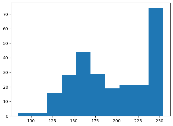
Modifying images
Thresholding and pixel manipulation
# Modifying an image

MY_THRESHOLD = 150

img_bw = img.copy()
img_bw[img_bw<MY_THRESHOLD]=0
img_bw[img_bw>=MY_THRESHOLD]=255

mw_showimg(img_bw, fontcol='red')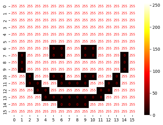
Managing image copies and references
# Illustration why img.copy
img2 = img.copy()
img3 = img2
img3[5:8,:] = 0
mw_showimg(img)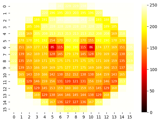
mw_showimg(img3)
mw_showimg(img2)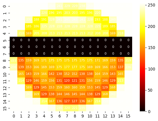
Conclusion: often, image.copy() is required. Some image-processing operations do not create a new, independent image, but instead return a view or reference to the same underlying data. This can cause unexpected behavior: changes made to the “processed” image also modify the original image. To avoid this, explicitly create a separate copy (for example, with image.copy()) before applying in-place edits. ### Multi-channel images
Working with RGB and multi-channel data
# Reading an RGB image
img_path_light = 'images/car/chatGPT_shadybusiness_zoomhigh-crop3.tif'
img_carlight = tiff.imread(img_path_light)
print("Image dimensions: ",img_carlight.shape)
_ = plt.imshow(img_carlight)
Image dimensions: (64, 59, 3)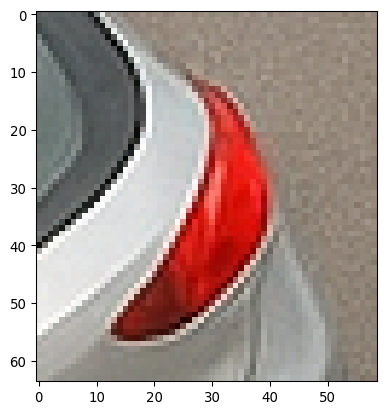
# Showing channels from a biology image

# Load the image
img_path_KTR = '/Users/m.wehrens/Data_notbacked/2025_Py-Image-workshop_KTR-example-data/raw/Composite_KTR.tif'
img_KTR = tiff.imread(img_path_KTR)

print("Image dimensions: ", img_KTR.shape)

# Display the three channels next to each other
fig, ax = plt.subplots(1,3)
_ = ax[0].imshow(img_KTR[0, 0, 0:200, 0:200], cmap='gray')
_ = ax[1].imshow(img_KTR[0, 1, 0:200, 0:200], cmap='gray')
_ = ax[2].imshow(img_KTR[0, 2, 0:200, 0:200], cmap='gray')
Image dimensions: (27, 3, 1024, 1024)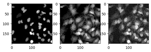
Saving images
Images can be saved using tiff.imwrite() for TIFF format or other libraries depending on the desired output format.
# Saving an image
tiff.imwrite('output-test/img_bw.tif', data=img_bw)
Exercises
- Read the image “images/car/chatGPT_shadybusiness_zoomhigh-custom.tif” and see if you can display it nicely.
- Can you display a zoom of the license plate?
- Can you similarly zoom and read the license plate in the image “chatGPT_shadybusiness_zoomlow-8bit.tif”?
- Try out some different
cmapvalues to display that same image.- What is an issue with e.g. the
hsvandjetcolormap, that e.g. theviridisandmagmacolormaps do not have?
- What is an issue with e.g. the
- What happens if we add 100 to the values in that image? I.e.
img_small_plus100 = img_small+100(Perhaps displayimg_small_plus100and investigate further.)
- Try out some different
Additional exercises
- Read the image “Composite_KTR.tif”, select the nuclear signal (channel 0), and:
- Use a histogram to determine a background/nuclei cutoff.
- Create a thresholded image.
- Using the function
plt.contour, carefully checking the documentation, draw nuclear outlines on top of the selected nuclear image.